Hello, dear friend, you can consult us at any time if you have any questions, add WeChat: daixieit

COMP 528

Continuous Assessment 2

Laplace equation solver

In this assignment, we will build a solver for the Laplace equation, which is a second-order Partial Differential Equation that appears in many areas of science and Engineering including electricity, fluid flow, and steady state heat conduction.

Here we will use the equation to model the steady state heat distribution in a room with a radiator. Although a real room is three dimensional, we will limit this exercise to two dimensions for simplicity. The room is 10 by 10m with a radiator along one wall as shown in Figure 1. The radiator is 4m wide and is centred along the wall, i.e. it takes up 40% of the wall, with 30% on either side. The radiator is held at a constant temperature of 100^◦C. The walls are all at 10^◦C. Together this specifies the temperature at every point at the boundaries of our domain (the room). Boundary conditions specified in this way are called Dirichlet boundary conditions.

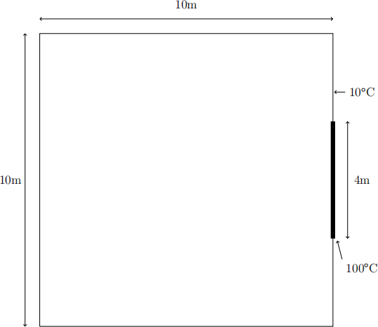
Figure 1: 10m × 10m room with a radiator

The steady-state heat distribution of this two-dimensional room can be found by solving the Laplace equation which, in its continuous form can be written as follows:

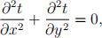
where t(x, y) is a continuous, twice-differentiable function describing the steady-state tem-perature at any point in the room, and , is the second partial derivative with respect to x, and similarly for y.

There are many ways to solving this partial-differential equation. Here we will solve it by dividing the area of the room in Figure 1 into a grid of points ti,j , to represent the temperature at the point (i, j) in the room. We can use the finite-difference method (and some simplifying assumptions) to express Equation 1 over this grid of points as:

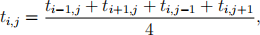
which is really just another way of saying that the temperature at any point is the average of the four points immediately around it.

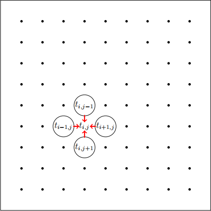
Figure 2: This problem is a stencil computation. The temperature value at every point can be calculated by averaging the temperature of its four neighbouring points.

This might remind you of something we studied in class - this is the famous stencil pattern (or a gather access), where every value in an array is calculated as a weighted sum of the points in its vicinity. This stencil is a simple one where the weights are the same. The example we saw in class was a one-dimensional stencil so each point had two neighbours. However, since this is a two-dimensional physical problem, instead of two neighbours, every point now has four neighbours. If we were to extend this problem to three dimensions (we will NOT do that here), every point would have six neighbours (two for each dimension). To simplify things, we will consider the points along the edge of our domain, i.e. where i = 0, j = 0, i = n, or j = n, to represent the walls, or the radiator. We will refer to these as the boundary points. All the points in the domain that are not boundary points will be called interior points, i.e. for 0 < i < n, 0 < j < n. In total there are (n + 1)² points, of which (n − 1)² are interior points while the rest are boundary points.

The temperature of the boundary points will be considered fixed. The temperature of the interior points will be calculated by using the formula given in Equation 2 iteratively until a given maximum number of iterations or when the temperature between successive iterations does not change by at least a given amount (whichever happens first).

Starter Code

We can store the temperature at each point in our domain in a two-dimensional array t[ i ][ j ]. The values in this array can be initialised as follows:

● The values of the points along the length of the radiator can be initialised as 100. These will be a subset of the boundary points on one of the boundaries (walls). If the radiator appears to end between two grid points, include the outer grid point in the radiator initialisation as well.

● All other points can be initialised at 10.

The rest of the program as a sequential code is given here:

for ( i = 1 ; i < n ; i++)

for ( j = 1 ; j < n ; j++)

r [ i ] [ j ] = 0.25 ∗ ( t [ i −1][ j ] + t [ i +1][ j ] + t [ i ] [ j −1] + t [ i ] [ j + 1] );

for ( i = 1 ; i < n ; i++)

for ( j = 1 ; j < n ; j++)

t [ i ] [ j ] = r [ i ] [ j ] ; // data copying

Note that this code will always run for a fixed number of iterations. It is up to you to implement an early termination criteria. Instead of dividing by 4, we multiply by 0.25 because computer systems usually implement floating-point multiplication as a faster operation than division. There are some inefficiencies in the given program - for example, we copy the results from r[ i ][ j ] back to t[ i ][ j ] at the end of each iteration. If you remember our discussion about the memory bottleneck, you will know that data movement is the enemy of program performance and should be minimised. Most things you can do to improve the serial performance of this code will also improve the performance of the parallel version so take your time to find inefficiencies in this code and improve it as you see fit while making sure that the numerical results don’t change.

All computations should be in double precision.

Task 1: Sequential Program

The given code can be improved by avoiding the data copying loop at the end of each iteration. This can be achieved by defining t as a three-dimensional array of size 2 ×(N + 1)×(N + 1), i.e. t[x][ i ][ j ]. Every iteration can then swap between reading from x=0 and writing to x=1, and vice-versa. For example, the first iteration could read from t [0][ i ][ j ] and write to t [1][ i ][ j ], while the second iteration could read from t [1][ i ][ j ] (which was just written in the previous iteration) and write to t [0][ i ][ j ] (overwriting the initial values since they are no longer required), and the third iteration would repeat what the first one did. Rewrite the given code to implement the above change to remove the extra data copy. Write a complete C program that models the temperature distribution of the room given in Figure 1. Your domain should consist of N × N points and you should solve to K iterations where N and K are defined constants in your code (so you can change them easily). Instrument the code to track the total time taken and display it in the end of the execution. Also display the final temperature at every N/8×N/8 points in your domain, i.e. 8 ×8 points, regardless of the value of N.

Use smaller values of N and K while developing and testing your code, but your submission should have N = 1024 and K = 100000.

Your submission for this task should include:

● Your sequential C program to solve the temperature distribution problem (as a .c file).

● A document containing:

– Screenshot of compiling the program on your computer

– Screenshot of the complete output of the program on your computer (could be for a smaller K and N.)

– Screenshot of compiling the program on Barkla.

– Complete program output (could be a screenshot) of the program on Barkla.

Task 2: OpenMP program

Modify the sequential program from Task 1 to be an OpenMP program. This program should start by solving the problem in serial (using the same code from Task 1), then it should solve the problem in parallel using OpenMP. It should also have code to check that the results do not change between the two invocations. Finally, measure the time for both versions, calculate and report both the times and the speedup achieved.

Your submission for this task should include:

● Your complete OpenMP program to solve the temperature distribution problem (as a .c file).

● A document containing:

– Screenshot of compiling the program on your computer

– Screenshot of the complete output of the program on your computer (could be for a smaller K and N.)

– Screenshot of compiling the program on Barkla.

– Complete program output (could be a screenshot) of the program on Barkla.

– A table showing the run times for 1, 2, 4, 8, 16 and 32 threads.

– A plot showing speedup vs number of threads (see Lecture05.pdf, slides 31/32 for an example).

Hints

You might get a segmentation fault trying to allocate an array like double t[2][N+1][N+1] on your computer or even Barkla for large values of N. This is because the previous statement allocates the memory on the stack, and there is a very tight limit on the size of variables you can allocate on the stack. Instead, you should allocate this on the heap using the following statement:

double (∗ t ) [N+1][N+1] = malloc ( sizeof (double [ 2 ] [ N+1][N+ 1 ] ) ) ;

In general, if you get segmentation faults when running your program, use a tool called gdb to help debug. Read its manual to understand how to use it.

OpenMP has some pragmas to help the compiler spot vectorisation opportunities. Read about them in the OpenMP manual.

My reference solution (which is not particularly optimised) took about 160 seconds on Barkla in serial execution, and a best time of about 12 seconds in parallel execution. Use these timings to guide your efforts.

You can consider printing the state of the domain every 500 iterations to follow the progress of your simulation. However, make sure to remove all print statements from inside the timed section when measuring runtime - the print statements will immensely slow down your program! The timings I gave above are with the prints removed.

Marking scheme and submission

Your submission should be a zip file containing two documents, and two .c files - one for each task above. Also include your SLURM submission scripts. This should be submitted on Canvas, as the submission for CA2 in COMP 528.

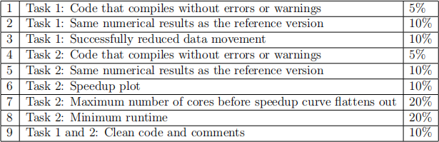
Table 1: Marking scheme

The purpose of this assessment is to develop your skills in analysing numerical programs, and developing OpenMP programs. This assessment contributes 13% to the overall mark in the module. The scores from the above marking scheme will be scaled down to reflect that. Failure in this assessment may be compensated for by higher marks in other components of the module. Submissions will be submitted to automatic plagiarism/collusion detection systems, and those exceeding a threshold will be reported to the Academic Integrity Officer for investigation regarding adhesion to the university’s policy https://www.liverpool.ac.uk/media/livacuk/tqsd/code-of-practice-on-assessment/appendix L cop assess.pdf.