STAT 603: Midterm Assignment
Hello, dear friend, you can consult us at any time if you have any questions, add WeChat: daixieit
STAT 603: Midterm Assignment
Due: Monday, April 1
Directions:
1. Turn in your midterm answers (including R source code) on Canvas as well as a hard copy in class.
2. Show all your work! Both source code and key outputs from running your code are required. Simply giving a final answer or source code without appropriate explanation/key outputs will not receive any points.
3. Typing answers in RMarkdown or LaTeX is strongly recommended.
4. You may work in groups to discuss about ideas, but the writing and programming must be your own work. Copying others’ work and code or allowing others to copy your own work will result in zero point for the midterm assignment.
Part 1
The following two problems are from the textbook Convex Optimization by BV, Chapters 4.1–4.3 (only subsections relevant to in-class instruction)
Q1. 4.1 (a)(b)(c)
Note: You should provide the graphical sketch of the feasible set, find the answer, and verify that your answer satisfies the optimality condition that
Δf0 (x)T (y − x) ≥ 0 for all feasible point y.
Q2. 4.15(a)
Part 2
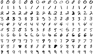
In the following we work on the MNIST database (Modified National Institute of Standards and Technology database). The original MNIST data contains 60,000 training images and 10,000 testing images, each containing the image of a handwritten single digit (0–9). The following picture contains a small subset of images from this data (picture from Wikipedia).
For our purpose of this assignment, a random sample of 10,000 training images and 5,000 testing images are taken (without replacement) from the original data sets. For each original image, there are 28 × 28 pixels that contain values from 0-255. We simply convert them into binary variables 0 and 1: if the original value is larger than 0, we use 1; otherwise it’s 0. As a result, the training data is saved as “mnist_train_binary.csv” and the testing data is saved as “mnist_test_binary.csv”. In both training and testing data sets, the first column gives the true digit label, and the remaining 784 columns corresponds to the binary variables. To understand this data better, let’s first load the data; then we look at the 10th row from the training data:
# load the data
traindat <- as.matrix (read.table ( "mnist_train_binary.csv" ,sep=","))
colnames (traindat) <- c ( "label" ,paste ( "x" ,1:784 ,sep= ""))
# read the n th data point
n <- 10
label <- traindat[n,1]
binvar <- traindat[n,2:785]
# print true digit label
label
## label
## 9
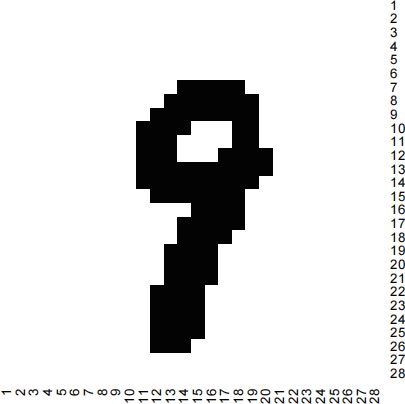
So the true label of this image is “9”. We can also convert the binary variable vector “binvar” to the 28 × 28 matrix pixels and visualize the image. A pixel with black color represents 1 and a pixel with white color represents 0.
# convert binvar to image matrix
matbin <- matrix (binvar,nrow=28 ,ncol=28 ,byrow=TRUE)
# draw a heatmap to visualize the image
heatmap (matbin,col=paste("gray" ,c (99 ,1),sep= ""),Rowv=NA ,Colv=NA ,revC=T)
Our ultimate goal is to use the training data set (including the true labels) to build a classification model and then make label predictions on the testing set. Note that when making label predictions, we only use the image variables in the testing set, but NOT the true labels. The true label in the testing set is only used to calculate the classification model’s prediction error/accuracy rate.
Before our attempt to build any model, let’s quickly explore these data sets a bit more. Answer the following questions.
Q1 In the training data set, find the last data point with true digit label “7”. Report its row number in the data and plot a heatmap to visualize its binary image variables.
Q2 In the testing data set, find the 200th data point and plot a heatmap to visualize its binary image variables. What is your guess on the true label? Does your guess (that is, an instant model built from the huge information collected from our life experience) match the true digial label?
(Hopefully, our human brain can build very accurate image classification model instantly. . . but imagine that you have to do it for tens of thousands of images. . . )
Q3 In the training data set, count the sample size for each digit label 0-9, and calculate their sample
proportions π(ˆ)k (k = 0, 1, · · · , 9). Make a table to report your counting/proportion results.
Next, let’s try to build a relatively “naive” probabilistic model from the training data. To begin with, we compress each image data point by dividing the 28 × 28 image pixels into 4 × 4 blocks and count the number of 1’s in each block. As a result, we obtain 7 × 7 count matrix. To store the count data, we vectorize it to a count vector x ∈ R49. After the data conversion to the counts, the compressed training data is saved as “mnist_train_counts.csv”, and the compressed testing data is saved as “mnist_test_counts.csv”. Their first columns are still the true digit labels, and the remaining 49 columns are the count vectors.
Before introducing the “naive” model, let’s first get familiar with these compressed data. For example, we can take a look at the 10th sample point in the compressed training data set.
# load the data
traindat1 <- as.matrix (read.table ( "mnist_train_counts.csv" ,sep=","))
colnames(traindat1) <- c ( "label" ,paste ( "x" ,1:49 ,sep= ""))
# read the n th data point
n <- 10
label <- traindat1[n,1]
cntvar <- traindat1[n,2:50]
# print true digit label
label
## label
## 9
As expected from before, the true digit label is still “9”. We can also convert the count vector to 7 × 7 matrix to visualize it with heat map:
# convert binvar to image matrix
matbin <- matrix (cntvar,nrow=7 ,ncol=7 ,byrow=TRUE)
# draw a heatmap
heatmap (matbin,col=paste("gray" ,99:1 ,sep= ""),Rowv=NA ,Colv=NA ,revC=T)
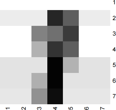
Not surprisingly, the image looks more blurred with compression, but the size of the image matrix is much less than the original one. Using the compressed data sets, answer the following questions.
Q4 In the compressed training data set, find the last data point with true digit label “7”. Report its row number in the data and plot a heatmap to visualize its count variables.
Q5 In the compressed testing data set, find the 200th data point and plot a heatmap to visualize its count variables. Print out the true digital label and verify if the digit label is the same as you obtained in Q2.
Q6 In the compressed training data set, count the sample size for each digit label 0-9, and calculate their
sample proportions π(ˆ)k (k = 0, 1, · · · , 9). Make a table to report your counting results. Verify if the sample
sizes and sample proportions are the same as you obtained in Q3.
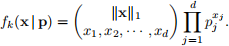
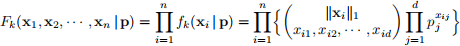
Next, using the compressed training data set, we are ready to introduce a multinomial probability model for digit k (k = 0, 1, · · · , 9). Let’s take the digit “7” for example (that is, k = 7). We assume that a count
vector x = (x1 , x2 , · · · , xd ) ∈ Rd , given its total count ∥x ∥ 1 = Σj(d)=1 xj , follows a multinomial distribution
with probability vector p = (p1 , p2 , · · · , pd ), where d = 49 is the length of the count vector and p satisifies
Σj(d)=1 pj = 1. Then recall from STAT 601 that the probability mass function (p.m.f.) of a multinomial distribution is
Then suppose we have independent sample with sample size n for the digit label k = 7. Denote the sample points by x1 , x2 , · · · , xn ∈ Rd with xi = (xi1 , · · · , xid ). Then we can write down the joint probability mass function for digit label k = 7 as
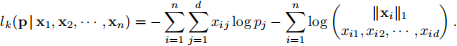
and its negative log-likelihood is
To find the maximum likelihood estimator (MLE) for the probability vector p associated with the multinomial distribution, we need to solve
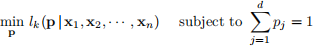
Q7 Is this MLE problem a convex optimization problem? Explain your answer.
Q8 Write down the Lagrangian function Lk (p, λ | x1 , x2 , · · · , xn ) of this MLE problem, where λ is the dual variable. Find the dual function and dual problem with respective to λ .
2024-03-25