Hello, dear friend, you can consult us at any time if you have any questions, add WeChat: daixieit

MMF1941H: Stochastic Analysis - Assignment # 1

1 Instructions

1. Please have your final report typeset using LATEX and submit your report individually. Provide code separate in a Python script file that you attach in your submission.

2. You may discuss these questions with your fellow students, however the write-up must be yours and yours alone, sharing of the write-up before the deadline is not allowed.

2 Problem: Bachelier Call Option Pricing

Let X be a standard normal random variable and let and variance  parameters. We are looking at the value of a call option in the Bachelier Model ie

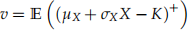
for a given strike K.

1. (10 pts) Show that for

holds where is the pdf of the standard normal distribution and the respective cdf. (Hint: you can exploit that holds).

2. (5 pts) Use the previous result to show that analytically

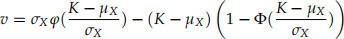
holds.

3. (10 pts) For a parameter we can define a measure via the definition

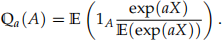
For calculate the and conclude that under X again follows a normal distribution and determine its parameters.

4. (5 pts) Write Python code to simulate the option value 1000 times under the measure P with a sample size of 5000 simulations each for and K = 8. Share the code and provide a histogram of the results. Also calculate the exact value analytically per the above formula.

5. (5 pts) Denoting vj a single MC estimate (based on 5000 simulations) for j = 1, . . . , M with M = 1000 we can define the sample variance as

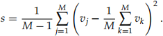
Calculate the sample variance for your previous experiment.

6. (10 pts) Note that for any a the option value can be re-written as

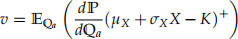
which mathematically will yield the same answer for any a. Define

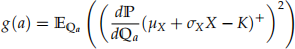
which can be evaluated through MC simulation given the fact the distribution of X under the measure is known. Write Python code plot the function g(a) for the above selection of parameters and Note that equivalently,

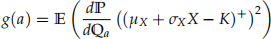
holds which you could use alternatively for implementation purposes.

7. (5 pts) Determine the minimum of the function g numerically (and approximately) from the prior plot and repeat the experiment of simulating the option value but now calculated through

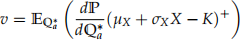
– where g attains its minimum at times with a sample size of 5000 simulations each and again determine the sample variance. Plot the histogram of this experiment again.