Hello, dear friend, you can consult us at any time if you have any questions, add WeChat: daixieit

STAT 231 Winter 2024

Assignment 4

Assignment 4 is due on Tuesday March 19 at 11:00am Eastern Time. Your assignment must be typed. You may create your document in Word, Google Docs, LaTeX or any other word processor. The requirement to type your assignment is to facilitate the grading so that the marked assignments can be returned to you in a timely fashion. It is also useful for you to gain some experience in creating a document containing mathematical expressions. Two documents have been posted in the Assignment 1 folder in LEARN on how to use the equation editor in Word. If you wish to use LaTeX then you may find Overleaf particularly useful for this. See https://www.overleaf.com/edu/uwaterloo

Upload your assignment to Crowdmark as a pdf file. You can upload your assignment as one document or individually for each problem. If you upload one document then you must drag and drop the pages for each problem to the appropriate question as indicated in Crowdmark. This is extremely important since dealing with assignments which are left as one document requires extra time and effort by the markers. Be sure to upload your assignment well in advance of the due time since uploading an assignment of many pages to Crowdmark requires time.

In addition to submitting your assignment component to Crowdmark, you must submit your assignment as a single pdf document to the Assignment 4 Dropbox in LEARN to facilitate the running of your assignment through plagiarism detection software. Your submissions to Crowdmark and the LEARN Dropbox must be identical. Please do not include these two pages of information or any instructions given for each problem in your assignment submission to Crowdmark and the LEARN Dropbox. Doing so means that your assignment is flagged by the Turnitin software used for checking plagiarism.

Many problems on this assignment indicate that your answers must be given in sentences. This course emphasizes learning to communicate statistical concepts in sentences.

In some of the problems on this assignment you are asked to use R.  Only the answers/results you obtain using R must be included in your Crowdmark pdf submission.  Your R code must be uploaded as an R file to the Assignment 4 R Code Dropbox in LEARN. Effectively commenting your code is a important skill to develop. Markers will review your file and run it to verify the answers match those in your Crowdmark submission and that the code runs without error. Your code must correctly find the answers needed to get the marks associated with the problems. Good commenting will allow the marker to more easily assign you a full score when reviewing your file. Please ensure your code submitted in the R file is well commented.   

Penalties:

(1) Answers which are not typed will not be marked and will receive a mark of zero.

(2) An assignment which is uploaded late to Crowdmark will be assigned a penalty of 5% per hour.

(3) An assignment which is left as a single document and not uploaded to the appropriate places in Crowdmark will be assigned a 10% overall penalty.

(4) An assignment which is submitted late to the Assignment 2 Dropbox in LEARN will be assigned a 5% overall penalty.

(5) If the file of R code is submitted late to the Assignment 2 R Code Dropbox in LEARN, then the assignment will be assigned a 5% overall penalty.

(6) Answers which are required to be written in sentences but are not in sentences will be assigned a 5% overall penalty.

(7) Assignments which include R code in the Crowdmark submission will be assigned a 5% overall penalty.

Checklist to complete for this assignment:

Upload the pdf of your assignment to Crowdmark by the deadline.

Upload the pdf file of your assignment to the Assignment 4 Dropbox in LEARN by the deadline.

Upload the R file of your R code to the Assignment 4 R Code Dropbox in LEARN by the deadline.

This assignment is based on the material in Chapters 1-5 of the STAT 231 Course Notes.

Assignment 4 Learning Outcomes

Here are the intended learning outcomes for this assignment component. Try to identify the learning outcomes which are achieved by each of the given problems.

Enjoy

· Perform a test of hypothesis for Binomial(n,θ), Poisson(θ), and Exponential(θ) models using a test statistic based on the asymptotic Gaussian pivotal quantity and a  likelihood ratio test.

· Perform a test of hypothesis for the parameter μ and the parameter σ in a Gaussian model.

· Observe the connection between confidence intervals, likelihood intervals and hypothesis tests.

· Observe how p-values vary as the hypothesized value and sample size vary.

In Problems 1-4 you will continue to analyse variates in your data set. Make sure that you use the same data set that you generated, saved, and uploaded to the LEARN Dropbox as part of the Prerequisite Assignment.

Your commented R code should only be included in the R file that you upload to the LEARN Dropbox. Do not include your R code in your answers submitted to Crowdmark. All written answers must be in full sentences. Please do not include any instructions in your assignment submission to Crowdmark or the LEARN Dropbox.

The R code given in Problems 1-4 is also available in a text file called Assignment 4 R code posted in the Assignment 4 folder on LEARN.

Note: When conducting a test of hypothesis you should use a two-sided test unless otherwise stated. Be sure to show how your p-value was determined. When stating a conclusion about a null hypothesis please use the guidelines in Table 5.1 of the Course Notes. In this course we do not accept/reject hypotheses. Such conclusions will be marked wrong.

Problem 1: Tests of hypothesis for Binomial model

The purpose of this problem is to test the hypothesis H₀ : S = S₀ for Binomial(n,S) data. See Sections 5.1 to 5.3 and Table 5.2 of the Course Notes.

In this problem you will examine the data for the variate Wearing.a.watch (Are you wearing a watch? Yes or no?) for students who are aged less than 13.

The following R code provides you with the information you need for doing this question.

# data are assumed to be in the matrix called dataset

# Age variate in column 5, Watch variate in column 20

watch<-dataset[,c(5,20)]  

watch<-watch[complete.cases(watch),]   

# Watch observations for students aged less than 13

watch.lt13<-watch$Wearing.a.watch[watch$Age<13]

table(watch.lt13)

# the possible values for the derived variate watch.lt13 are yes, no and blank (missing)

(a) Include the following completed sentences in your assignment:

   (i) My student ID number is  __________.

   (ii) The variate Wearing.a.watch is a __________ variate.

   (iii) The number of observed values (that is, the observations were not missing) for the variate Wearing.a.watch for students aged less than 13 in my data set is n  __________.

Define the new variate yi = 1 if student i indicated “yes” that they are wearing a watch and yi= 0 otherwise, i = 1,2, ..., n. Let

   (iv) Complete the sentence: The value of y for my data set is __________.

    (v) The transformed variate y is a __________ variate.

(b) Describe a suitable study population for the empirical study which you have been conducting on the assignments and for which the sampling protocol consisted of downloading a data set from the CensusAtSchool New Zealand 2021website.

Let the random variable Y be the number of students aged less than 13 who are wearing a watch. For parts (c) and (d) assume that Y has a Binomial(n,θ) distribution.

(c)  (i) The parameter θ corresponds to what attribute of interest in the study population?

  (ii) What is the maximum likelihood estimate of θ for your data set?

(d) Watch retailers in New Zealand believe that 30% of students aged less than 13 in New Zealand wear a watch. You are interested in whether the percentage of students aged less than 13 who wear a watch in the study population in (b) is also 30%.

  (i) The asymptotic Gaussian test statistic for testing H₀: θ = θ₀ for a Binomial (n, θ) model is

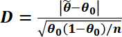
For your data what is the observed value d of this test statistic for the hypothesis H₀: θ = 0.3?

  (ii) Use the value of d determined in (d)(i) and the approximate Gaussian distribution of the test statistic D to determine the approximate p-value for testing H₀: θ = 0.3. Indicate clearly how the approximate p-value is determined. State your conclusion regarding this hypothesis based on the approximate p-value.

  (iii) Is the value θ = 0.3 an element of an approximate 99% confidence interval for θ based on the asymptotic Gaussian pivotal quantity? Explain why or why not using only the p-value determined in (d)(ii).

  (iv) For your data what is the observed value λ(θ₀) of the likelihood ratio statistic for testing the hypothesis θ₀ = 0.3?

The following R code will calculate the likelihood ratio statistic for a test of the null hypothesis that theta = theta0 for the Binomial model if the maximum likelihood estimate of theta is thetahat and the sample size is n:

lambda<-2*n*(thetahat*log(thetahat/theta0)+ (1-thetahat)*log((1-thetahat)/(1-theta0)))

  (v) Use the value of λ(0.3) determined in (d)(iv) and the asymptotic distribution of the likelihood ratio statistic to determine the approximate p-value for testing H₀: θ = 0.3. Indicate clearly how the approximate p-value is determined.  State your conclusion regarding this hypothesis based on the approximate p-value.

  (vi) Is your conclusion in (d)(v) the same as your conclusion in (d)(ii)? Briefly explain why you would (or would not) expect these conclusions to be the same.

 (vii) Is the value θ = 0.3 an element of a 50% likelihood interval for θ? Explain why or why not without determining the likelihood interval.

Problem 2: Tests of hypothesis for Poisson model

The purpose of this problem is to test the hypothesis H₀ : S = S₀ for Poisson(S) data. See Sections 5.1 to 5.3, and Table 5.2 of the Course Notes.

In this problem you will examine the data for the variate Jeans (How many pairs of jeans do you have? (Jeans are long pants made of denim. They can be any colour.) for students aged greater than 13.

The following R code stores the subset of observations used in this analysis in the vector jeans.gt13:

# data are assumed to be in the matrix called dataset

# Age variate in column 5, Jeans variate in column 18

jeans.data<-dataset[,c(5,18)]

jeans.data<-jeans.data[complete.cases(jeans.data),]    # analyze only complete cases

# subset of data for students aged greater than 13

jeans.gt13<-jeans.data$Jeans[jeans.data$Age>13]

table(jeans.gt13)

(a) Include the following completed sentences in your assignment:

   (i) My student ID number is  __________.

   (ii) The variate Jeans is a __________ variate.

   (iii) The number of observations in my data set for the variate Jeans for students aged greater than 13 who responded to this question is  n = __________.

(b) To analyse the observations in the vector jeans.gt13 assume that they represent a random sample from a Poisson (θ) model.

  (i) The parameter θ corresponds to what attribute of interest in the study population?

  (ii) The sample mean for my data set is  ___________________.

  (iii) The sample variance for my data set is ____________.

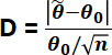
  (iv) Complete the following table of observed and expected frequencies assuming a Poisson model for the observations in the vector jeans.gt13. For convenience, expected frequencies may be rounded to 3 decimal places.

Whenever a model is assumed for a data set it is very important to check that the model fits the data since the point and interval estimates and the hypothesis tests depend on this assumption. If the model is not correct, the conclusions may be incorrect.

(v) Based on the numerical summaries above, how well would you say the Poisson model fits your data? Be sure to justify your answer. (See page 92 of the Course Notes.)

Note: Even if you conclude the Poisson model does not fit your data well, continue to do the analyses in (c) based on the Poisson model. Note that this would not be done in a real world analysis!

(c) Jeans retailers in New Zealand have hypothesized that students aged greater than 13 have on average three pairs of jeans. You are interested in whether the mean number of jeans that students aged greater than 13 in the study population for this study have equals 3.

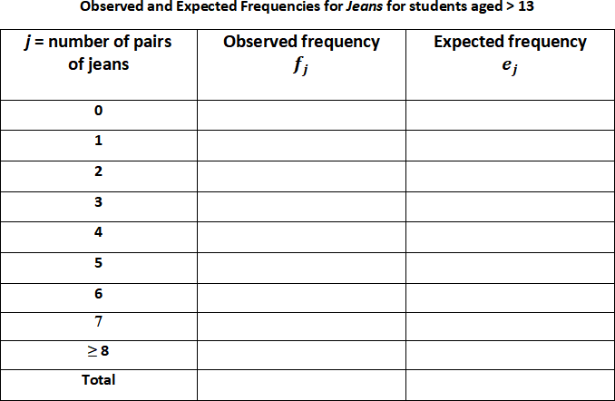
  (i) The asymptotic Gaussian test statistic for testing H₀: θ = θ₀ for a Poisson (θ) model is

For your data what is the observed value d of this test statistic for the hypothesis H₀: θ = 3?

  (ii) Use the value of d determined in (c)(i) and the approximate Gaussian distribution of the test statistic D to determine the approximate p-value for testing H₀: θ = 3. Indicate clearly how the approximate p-value is determined. State your conclusion regarding this hypothesis based on the approximate p-value.

  (iii) For your data what is the observed value λ(θ₀) of the likelihood ratio statistic for testing the hypothesis H₀: θ = 3?

The following R code will calculate the likelihood ratio statistic for a test of the null hypothesis that theta = theta0 for the Poisson model if the maximum likelihood estimate of theta is thetahat and the sample size is n:

lambda<-2*n*(thetahat*log(thetahat/theta0)+(theta0-thetahat))

  (iv) Use the value of λ(3) determined in (c)(iii) and the asymptotic distribution of the likelihood ratio statistic to determine the approximate p-value for testing H₀: θ = 3. Indicate clearly how the approximate p-value is determined. State your conclusion regarding this hypothesis based on the approximate p-value.

  (v) Is your conclusion in (c)(iv) the same as your conclusion in (c)(ii)? Briefly explain why you would (or would not) expect these conclusions to be the same.

Problem 3: Tests of hypothesis for Exponential model

The purpose of this problem is to test the hypothesis H₀ : S = S₀ for Exponential(S) data. See Sections 5.1 to 5.3, and Table 5.3 of the Course Notes.

In this problem you will examine the data for the variate Travel.time.to.school. (How long does it usually take you to get to school? Answer to the nearest minute.) for students aged great than 14.

The following R code stores the subset of observations used in this analysis in the vector time.travel.gt14:

# data are assumed to be in the matrix called dataset

# Age variate in column 5, Travel.time.to.school variate in column 30

time.travel<-dataset[,c(5,30)]

time.travel<-time.travel[complete.cases(time.travel),]   # analyze only complete cases

# subset of data for students aged greater than 14

time.travel.gt14<-time.travel$Travel.time.to.school[time.travel$Age>14]

summary(time.travel.gt14)

(a) Complete the following statements:

   (i) My student ID number is  __________.

   (ii) The variate Travel.time.to.school is a __________ variate.

   (iii) The number of observations in my data set for the variate Travel.time.to.school for students aged greater than 14 who responded to this question is  n = __________.

(b) To analyse the observations in the vector time.travel.gt14 assume that they represent a random sample from a Exponential (θ) model.

  (i) The parameter θ corresponds to what attribute of interest in the study population?

  (ii) The sample mean for my data set is  ___________________.

  (iii) The sample standard deviation for my data set is ____________.

  (iv) Use R to plot the empirical cumulative distribution function with the appropriate superimposed Exponential cumulative distribution function for the observations in the vector time.travel.gt14.

To receive full marks:

· plot must occupy 1/3 to 1/2 of a page both vertically and horizontally

· plot must have title

· axes must be labeled

· plot must include a legend

· the range of x and y values must be chosen such that the empirical cumulative distribution function and the superimposed Exponential cumulative distribution function are both fully visible

Whenever a model is assumed for a data set it is very important to check that the model fits the data since the point and interval estimates and the hypothesis tests depend on this assumption. If the model is not correct, the conclusions may be incorrect.

  (v) Based on the numerical and graphical summaries above, how well would you say the Exponential model fits your data? Be sure to justify your answer. (See pages 92 and 93 in the Course Notes.)

Note: Even if you conclude the Exponential model does not fit your data well, continue to do the analyses in (c) based on the Exponential model. Note that this would not be done in a real world analysis.

In 2011 the average travel time to school for all students aged greater than 14 in the study population was 25 minutes. You are interested in whether the mean travel time for students aged greater than 14 in the study population for this study is still 25 minutes.

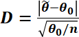
(c) (i) The asymptotic Gaussian test statistic for testing H₀: θ = θ₀ for a Exponential (θ) model is

For your data what is the observed value d of this test statistic for the hypothesis H₀: θ = 25?

  (ii) Use the value of d determined in (c)(i) and the approximate Gaussian distribution of the test statistic D to determine the approximate p-value for testing H₀: θ = 25. Indicate clearly how the approximate p-value is determined. State your conclusion regarding this hypothesis based on the approximate p-value.

  (iii) For your data what is the observed value λ(θ₀) of the likelihood ratio statistic for testing the hypothesis H₀: θ = 25?

The following R code will calculate the likelihood ratio statistic for a test of the null hypothesis that theta = theta0 for the Exponential model if the maximum likelihood estimate of theta is thetahat and the sample size is n:

lambda<-2*n*(log(theta0/thetahat)+(thetahat/theta0-1))

  (iv) Use the value of λ(25) determined in (c)(iii)and the asymptotic distribution of the likelihood ratio statistic to determine the approximate p-value for testing H₀: θ = 25. Indicate clearly how the approximate p-value is determined. State your conclusion regarding this hypothesis based on the approximate p-value.

  (v) Is your conclusion in (c)(iv) the same as your conclusion in (c)(ii)? Briefly explain why you would (or would not) expect these conclusions to be the same.

  (vi) For your data what is the observed value d₁ of the exact test statistic

for testing the hypothesis H₀: θ = 25?

  (vii) Use the value of d₁ determined in (c)(vi) and the exact distribution of D₁ to determine the exact p-value for testing H₀: θ = 25 (see Table 5.3 in the Course Notes). Indicate clearly how the exact p-value is determined. (Use the R command pchisq for your calculation.) State your conclusion regarding this hypothesis based on the p-value.

  (viii) Is your conclusion in (c)(vii) the same as in (c)(ii)? Briefly explain why you would (or would not) expect these conclusions to be the same.

Problem 4: Tests of hypotheses for Gaussian data

The purpose of this problem is to test the hypotheses for Gaussian data. See Sections 5.1 to 5.3, and Table 5.3 of the Course Notes.

In this problem you will examine the data for the Bag.weight variate (What is the weight of your school bag today? Answer in kilograms to one decimal place. (Weigh your school bag with all your books and other materials you brought to school today.)) for students aged 15.

The following R code stores the subset of observations used in this analysis in the vector bagweight.15:

# data are assumed to be in the matrix called dataset

# Age variate in column 5,  Bag weight variate in column 31

bagweight<-dataset[,c(5,31)]

bagweight<-bagweight[complete.cases(bagweight),]   # analyze only complete cases

# subset of data for students aged 15

bagweight.15<-bagweight$Bag.weight[Bag.weight$Age==15]

summary(bagweight.15)

(a) Complete the following statements:

   (i) My student ID number is  __________.

   (ii) The variate Bag.weight is a __________ variate.

   (iii) The number of observations in my data set for the variate Bag.weight for students aged 15 who responded to this question is  n = __________.

(b) To analyse the observations in the vector bagweight.15 assume that they represent a random sample from a G(μ, σ) model.

  (i) The parameter μ and σ correspond to what attributes of interest in the study population?

  (ii) The sample mean for my data set is  ___________________.

  (iii) The sample standard deviation for my data set is ____________.

  (iv) The sample skewness for my data set is ____________.

  (v) The sample kurtosis for my data set is ____________.

  (vi) Give a qqplot for this variate.

Whenever a model is assumed for a data set it is very important to check that the model fits the data since the point and interval estimates and the hypothesis tests depend on this assumption. If the model is not correct, the conclusions may be incorrect.

  (vii) Based on the numerical and graphical summaries above, how well would you say the Gaussian model fits your data? Be sure to justify your answer.

Note: Even if you conclude the Gaussian model does not fit your data well, continue to do the analyses in (c) and (d) based on the Gaussian model. Note that this would not be done in a real world analysis.

(c) In 2011 the average bag weight was 5 kilograms for all the students in the study population aged 15. You are interested in whether the mean bag weight for students aged 15 in the study population for this study is still 5 kilograms.

  (i) Use your data to test the hypothesis H₀ : μ = 5.

Be sure to state the observed value of the test statistic

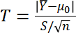
the corresponding p-value, and your conclusion based on this p-value. Explain how the p-value is determined by the R function t.test.

Note: To test hypotheses about the mean for a Gaussian model you can use the R command t.test(). See Chapter 5, Problem 3, for an example. You can also access specific results from using the t.test() command directly. For example, to test the null hypothesis that the mean of a Gaussian distribution is 3 for a sample called y, you use the R command  

t.test(y, mu = 5)$p.value

and R returns the p-value specifically. You can also use $statistic and $parameter in a similar manner.

  (ii)  Is the value μ = 5 an element of a 90% confidence interval for μ? Explain why or why not using only the p-value determined in (c)(i).

(d) (i) Use your data to test the hypothesis H₀ : σ = 3.

Be sure to state the observed value of the test statistic

the corresponding p-value, how the p-value is determined, and your conclusion based on this p-value.

  (ii) Is the value σ = 3 an element of a 99% confidence interval for σ? Explain why or why not using only the p-value determined in (d)(i).

Problem 5: Tests of hypotheses and shiny app

Go to the shiny app: https://shiny.math.uwaterloo.ca/sas/stat231/teststatistics/ 

You can use this app to explore test statistics and hypothesis tests. You can first choose a probability distribution and a test statistic. You then specify a value for the model parameter under the null hypothesis. You can then adjust the sample size, and set the point estimate of the model parameter resulting from the sample. The right-hand window then displays a plot of the probability distribution corresponding to the test statistic chosen. The plot is then separated into regions based on the value of the resulting test statistic. You should think about how the areas under the probability distribution curves correspond to the resulting p-values.

Part A: Binomial(n, θ)

Recall that the asymptotic Gaussian test statistic for the Binomial(n,θ) model is

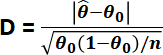
(a) On the shiny app select Binomial as the distribution, Asymptotic Gaussian as the test statistic, 0.1 as the H₀ value for θ, and 30 as the sample size. As you move the slider for MLE of θ, you will see how the value of the test statistic and the corresponding p-value for testing H₀: θ = 0.1 vary as the value of  varies.

 (i) Use the shiny app to complete Table 1.

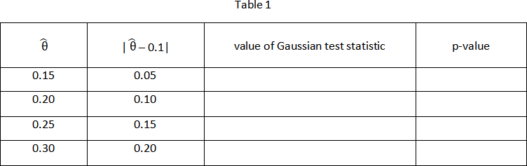
 (ii) How does the p-value for testing H₀: θ = 0.1 change as the quantity | – 0.1| increases? Give a statistical (not mathematical) argument why this behaviour makes sense.

 (iii) What other value of  generates the identical test statistic and p-value as when

| – 0.1| = 0.05? Explain mathematically why this happens.

(b) On the shiny app select Binomial as the distribution, Asymptotic Gaussian as the test statistic, 0.1 as the H₀ value for θ, and 0.15 as the MLE of θ. As you change the value of the sample size, you will see how the value of the test statistic and the corresponding p-value for testing H₀: θ = 0.1 vary as the value of the sample size varies.

  (i) Use the shiny app to complete Table 2.

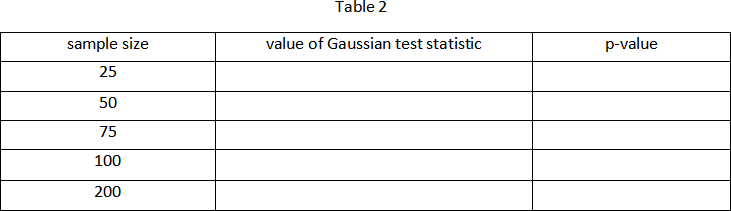
 (ii) How does the p-value for testing H₀: θ = 0.1 change as the sample size increases for a fixed value of  ? Give a statistical (not mathematical) argument why this behaviour makes sense.

(c) On the shiny app select Binomial as the distribution, Likelihood ratio as the test statistic, 0.1 as the H₀ value for θ, and 30 as the sample size. As you move the slider for MLE of θ, you will see how the value of the test statistic and the corresponding p-value for testing H₀: θ = 3 vary as the value of  varies.

  (i) Use the shiny app to complete Table 3.

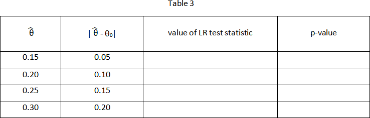
  (ii) Compare the p-values in Table 3 with the p-values in Table 1. If you use Table 5.1 as your guide for conclusions, is there any value of  in Table 1 which gives a different conclusion regarding the hypothesis H₀: θ = 0.1 for the same value of  in Table 3?

Part B:  Gaussian standard deviation σ

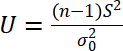
Recall that the test statistic for testing the hypothesis H₀ : σ = σ0 for the Gaussian model is

(a) On the shiny app select G(μ,σ) as the distribution, Standard deviation (σ) as the Test for mean or standard deviation, 4 as the H₀ value for σ, and 30 as the sample size, 1 as the sample mean, and 4.4 as the sample standard deviation. As you move the slider for the sample standard deviation, you will see how the value of the test statistic and the corresponding p-value for testing H₀: σ = 4  vary as the value of the sample standard deviation varies.

  (i) Use the shiny app to complete Table 4.

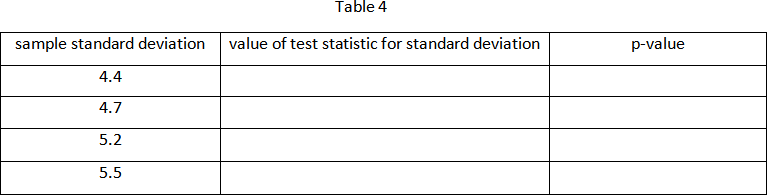
 (ii) How does the p-value for testing H₀: σ = 4  change as the sample standard deviation increases for a fixed value of the sample mean and the sample size? Give a statistical (not mathematical) reason why this behaviour makes sense.

(b)

 (i) On the shiny app select G(μ,σ) as the distribution, Standard deviation (σ) as the Test for mean or standard deviation, 3 as the H₀ value for σ, and 30 as the sample size, 0 as the sample mean, and 2 as the sample standard deviation. Record the value of the test statistic and p-value for testing H₀: σ = 3.

 (ii) On the shiny app select G(μ,σ) as the distribution, Standard deviation (σ) as the Test for mean or standard deviation, 6 as the H₀ value for σ, and 30 as the sample size, 0 as the sample mean, and 4 as the sample standard deviation. Record the value of the test statistic and p-value for testing H₀: σ = 6.

  (iii) What do you notice about the values of the test statistic and p-value for these two cases? Explain mathematically why this happens.

(c) On the shiny app select G(μ,σ) as the distribution, Standard deviation (σ) as the Test for mean or standard deviation, 2 as the H₀ value for σ, and 30 as the sample size, -3 as the sample mean, and 2.5 as the sample standard deviation. As you move the slider for the sample mean, you will see how the value of the test statistic and the corresponding p-value for testing H₀: σ = 2  vary as the value of the sample mean varies.

  (i) Use the shiny app to complete Table 5.

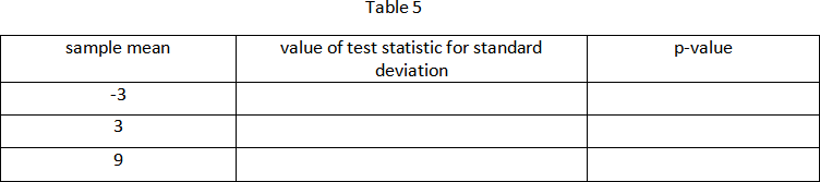
  (ii) How does the p-value for testing H₀: σ = 2  change as the sample mean increases for a fixed value of the sample standard deviation and the sample size? Explain mathematically why this happens.