Week 4 Jupyter Notebook Written Report Statistical Processes
Due date: Sunday of Week 5
Grading & Weight: This assignment is out of 100 marks, as further specified in the mark breakdown foreach question, and in the rubric below. The assignment is worth 9.5% of your overall final grade in the course.
Late Penalty: Late submissions will be penalized at 10% each day for up to 5 days, in which case a grade of zero will be given.
1. Overview
For this assignment, you will model a number of processes to help you get a better understanding of random processes. You will answer 4 questions that will help you better understand these processes. You will submit a report to onQ in the form of a Jupyter notebook before the deadline specified.
This assignment directly aligns with the following Course Learning Outcomes (CLOs):
CLO 2: Explain random processes, including Gaussian, Poisson and binomialCLO 3: Analyze random processes, including Gaussian, Poisson and binomial
1.1 Time for completion
This assignment will take approximately six (6) hours to complete. You will begin working on this assignment in the two hour tutorial of Week 4, and finish on your own time before the deadline.
1.2 Instructions
For this assignment, you will answer the questions in order to improve your understanding of the content that you have become familiar with this week. You will submit a report in the form of a Jupyter notebook. Your Jupyter notebook must contain the following information:
- Completion of the tasks and discussion
- Include code required to correctly complete the task
- Include comments to explain your thought process and code logic
- Discuss the results of what was found and answer the questions in the task list
- Format
- See the Jupyter Notebook report template in onQ to format your report.
TASKS
Question 1
Context:
Take for the outcome of a hockey game, a win or a loss. Imagine a good team vs. a poor team. A good team will have a higher probability of winning games (P=0.7) compared to the poor team (P=0.3) while a middle of the pack team may have a win pct. of 50% (P=0.5). Now consider how these probabilities will play out over the course of a single game, a lockout shortened season (42 games), and a full 82 game season.
Steps:
1. Create a routine that uses a uniform random generator, from 0 to 1. For each game, draw a random number. If the number is smaller than P, suppose that the team won a game. If not, it lost. (use np.random.random, not a scipy.stats built-in distribution ) (3 marks)2. Let’s consider individual games. Using the “simulator” developed in step 1, simulate 100 independent games, using
a. P = 0.3 (2 marks)b. P = 0.5 (2 marks)c. P = 0.7 (2 marks)
3. Draw three histograms, one for each value of P. Plot the number of times you counted a win and the number of times you counted a loss. (2 marks)4. Now, instead of simulating individual games, simulate 100 seasons, each with 42 games, using
a. P = 0.3 (2 marks)b. P = 0.5 (2 marks)c. P = 0.7 (2 marks)
5. Draw three histograms of the number of games won in each season, one for each value of P.6. Simulate 100 seasons, each with 82 games, using
a. P = 0.3 (2 marks)b. P = 0.5 (2 marks)c. P = 0.7 (2 marks)
7. Draw three histograms of the number of games won in each season, one for each value of P. (2 marks)8. Up until now, you’ve drawn 9 histograms. Using a scipy.stats built-in distribution, overlay the appropriate distribution function over each histogram. (2 marks)9. Last year, the Toronto Maple Leafs won 46 games. Calculate the probability that, over an 82- game season, an average-strength team (P=0.5) wins 46 games or more. (2 marks)10. During the 2015-2016 season, the Montreal Canadiens started the season with 9 consecutive wins.
a. Calculate the probability for an average team (P=0.5) to win 9 games in a row. (2 marks)b. Later that year, the team lost 21 out of 26 games. Calculate the probability for an average team (P=0.5) to win 5 games or less out of 26 games. (2 marks)c. What random process did you use to answer (a) and (b)? What are the conditions for this process to be valid (i.i.d.)? Do you think that these conditions were met? (2 marks)
Question 2
Context:
Let’s think some more about hockey. More specifically, we’ll focus on the number of goals that a team will score in a game.
Steps:
1. Suppose that a team scores, on average, 3 goals per game.
a. What is the rate of goal-scoring per second? (2 marks)b. What is the rate of goal-scoring per second if the team scores, on average, 4 goals per game? (2 marks)c. What is the rate of goal-scoring per second if the team scores, on average, 5 goals per game? (2 marks)
2. Build a Python method that generate a uniform random number from 0 to 1 for every second of game played. If number is smaller than the rate, then a goal is scored. Each game is 60 minutes long. Simulate 82 games. (Use np.random.random, do not use scipy.stat ) Draw a histogram of the number of goals scored each game, the team scores, on average,
a. 3 goals per game (3 marks)b. 4 goals per game (3 marks)c. 5 goals per game (3 marks)
3. Using scipy.stat, generate random distributions which capture the simulations perform in step 2.Overlay these distributions over the histograms. (2 marks)4. How well do the distributions capture the histograms? What could be done to improve thematch between the distributions and the simulations? (2 marks)5. Jan Bulis, a former Montreal Canadien player, scored, on average, 0.17 goals per game.
a. What is the probability for him to score 4 goals in a game? (2 marks)b. In 2006, he scored 4 goals. How would you interpret this result? (2 marks)
Question 3
Context:
Enough with hockey. Let’s consider the production of a television. No two will likely be made the same but they will all generally fall within a set tolerance window in the manufacturing process. They will also be classified under the same energy star efficiency rating in which some tv's are more efficient than the guideline and some are less. Let’s suppose that the power consumption of the TVs is normally distributed. There are three processes to manufacture the TVs (process A, process B and process C). Process A has a mean of 60 W and a standard deviation of 10 W. Process B has a mean of 60 W and a standard deviation of 5 W. Process C has a mean of 55 W and a standard deviation of 10 W.
Steps:
1. For each process, you take 5 TVs and measure their power consumption. Use the function np.random.normal to generate 5 data points using each process. (1 mark)
a. By looking at the histogram, can you tell which process was used to generate each dataset? (2 marks)b. What if you measured 100 samples? (2 marks)c. What if you measured 1000 samples? (2 marks)
2. Use the scipy.stat.norm method to generate continuous distributions. Overlay them to the histograms generated in step 1. (2 marks)
Question 4
Context:
Not all data sets contain data in the shape of a standard distribution. Take for example a manufacturing process which requires a machine to be calibrated at the start of each day. If this machine is calibrated too far in either direction from 0 offset then every part produced in that day will be slightly over or undersized. This can lead to a double peaked Gaussian distribution.
Steps:
1. Let’s generate some data!
a. Create a numpy array using np.random.normal, with process mean -2, standard deviation 1.0, and size 10000. (2 marks)b. Create a numpy array using np.random.normal, with process mean 2, standard deviation 0.2, and size 2000. (2 marks)c. Concatenate (using np.concatenate) the two arrays. Congrats, you now have data! (2 marks)d. Plot a histogram of this data. (2 marks)
2. Can we provide a “smooth” representation of this concatenated data? Yes. There are a few ways to do this. Here, let’s use a Gaussian kernel density estimate (scipy.stats.gaussian_kde). Plot the Gaussian kernel density estimate. What does it represent? (2 marks)
3. Consider the concatenated array.
a. Calculate its standard deviation. (2 marks)b. Draw 4 random data points from it. This is a sample of size n=4. (2 marks)c. Calculate the sample mean of the sample drawn in step 3-b. (2 marks)d. Now, draw 5000 samples, each of size n=4. Calculate the mean of each of these samples (i.e. you’ll have 5000 means). Draw a histogram of these means. (2 marks)e. Calculate the standard deviation of these 5000 sample means. (2 marks)f. Draw 5000 new samples, each of size n=24 Calculate the mean of each of these samples (i.e. you’ll have 5000 means). Draw a histogram of these means. (2 marks)g. Calculate the standard deviation of these 5000 sample means. (2 marks)h. Compare the standard deviations calculated in 3-e and 3-g to the analytical formula of the standard error of the mean. (2 marks)
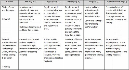
In addition to the marks above, your assignment will be evaluated using the following criterion:
2020-02-01