Instructions

General instructions:

. This is an individual project.  It consists of two parts and is worth 35% of the marks for this course. Please complete both parts.

.  This project is due on Monday, 25 March 2024.  Please submit your work on Learn. The submission deadline is 12:00 pm.  Any submission received after the deadline will incur a default late penalty.

.  Please note that the project has a  15-page limit for texts, tables, figures, other related outputs, and references  (but not including do files).   Each part provides some guidance on page allocation. Because marks are not awarded for the amount written, you do not need to aim for this page limit (10 pages are likely enough).

Instructions on presentation:

.  Please include relevant estimated regression equations, figures, and tables in the main body of your document.  In terms of regression outputs, you are encouraged to type out the equations rather than pasting Stata outputs directly.  For example, if Stata produces the following output for an AR(1) model

.  reg  p  L.p

Source  |               SS                       df              MS             Number  of  obs       =          1,304

-------------+----------------------------------    F(1,  1302)            =   40302.75

Model  |     1.00989004                  1    1.00989004      Prob  >  F                =         0.0000

Residual  |     .032624992          1,302    .000025058      R-squared              =        0.9687

-------------+----------------------------------      Adj  R-squared      =        0.9687

Total  |     1.04251503          1,303     .000800088      Root  MSE                =        .00501

you can present the equation as

 = 0.0180*** + 0.9844***pt−1 .

(0.0056)              (0.0049)

T = 1304, R2  = 0.9687

Alternatively, you can present a table with different sets of estimates, for example:

* p<0.10.  ** p<0.05.  *** p<0.01.

. Equations, figures, or tables that you refer to should be appropriately and informa- tively labelled. For figures, please include axis titles and legend when appropriate.

.  State the significance level when you conduct a hypothesis test.

.  Make sure that you are aware of the requirements for appropriate citation of ref- erences and data sources.  Read the guidance on plagiarism in Section 4.4.1 of the Economics Honours Handbook and/or the general University guidance.  If you in- clude anything from another source it must be properly acknowledged, whether it’s a figure/table or a text passage or anything else.

.  Please format everything such that the marker can easily mark your work.  (For instance, please avoid using small fonts and single spacing.)

.  Penalty may be imposed on poorly presented work.

Instructions on do files:

.  Please include the do file in your submission. Projects submitted without a do file will incur the default penalty of a late submission.

. The do file should be written in such away that anyone with access to the raw data files can replicate the analysis.

. You are welcome to complete this project using other statistical software.  The same rules apply: Please submit an executable script and include relevant output in the manuscript.

Part A

Note:   This part  is  worth  12%  of the final grade.   It  is  recommended  that you  allocate around three to four pages to this part.

Testing for unit root is crucial in financial econometrics, for many financial series contain unit roots that can affect statistical inference.  In class, we examined the Dickey-Fuller framework.  The framework has been extended in various ways since its introduction. Examples include

. allowing for structural breaks;

. different approaches to detrending the data;

. testing with stationarity as the null hypothesis.

Write a short essay (around 3–4 pages) on an extension(s) of the Dickey-Fuller framework. The essay can take one of the following broad and not necessarily mutually exclusive forms:

. An empirical analysis of a specific extension(s);

. A theoretical analysis of a specific extension(s);

. A literature review of the extensions proposed to date;

. A proposal of an extension(s) that fills a gap in the literature.

Some general guidelines:

.  Section 5.4 in the textbook provides a good starting point.

. Use appropriately defined mathematical notations when applicable.

.  Explain how the extension(s) complements the Dickey-Fuller framework.

. Discuss the limitations of the extension(s).

. Explore existing (or potential) applications of the extension(s).

Part B

Note:  This part is worth 23% of the final grade with each question weighted equally.  It is recommended that you allocate around one to two pages to each question.

Set-up:  For this part, you are invited to choose an exchange rate series for a pair of currencies.   Examples  include  GBP/EUR  (British pound to Euro) or USD/JPY  (US dollar to Japanese yen).

Sample period: You can decide which sample period to use, but the sample period should include an event (such as the COVID-19 pandemic) for later analysis.  A good rule would be to use 5 years of daily exchange rate data.

Data:  You can download the daily exchange rate series from http://finance.yahoo. com.  (See “Obtaining Yahoo Finance Data” below for instructions.)

Time series: You will be working with two time series, the exchange rate series and the return series.  You can treat closing prices as the exchange rate series.  Then, construct the return series using either the simple return formula or the log return formula.

B1.  Provide appropriate descriptive statistics of the exchange rate series you have cho- sen to study.  Does your series exhibit characteristics that conform to the stylised facts of financial returns data?

B2.  Use an appropriate model to produce ex ante forecasts for  exchange  rate  5  days ahead. Why have you chosen this model?

B3.  Calculate the 1% value at risk for the return series using the historical simulation method and the variance method. Comment on these value at risks.

B4.  Conduct an event study on the  return  series  using your  choice of event.   Com- ment on your results.  (For example, in response to COVID-19, Bank of England announced its £200 billion asset purchase plan on  19  March 2020—how does it affect GBP/EUR returns? Similarly, you can pick any event that could affect your currency pair.)

Obtaining Yahoo Finance Data

In this section, you can find basic instructions on how to download prices data from Yahoo Finance.

1.  Go to https://finance.yahoo.com/.

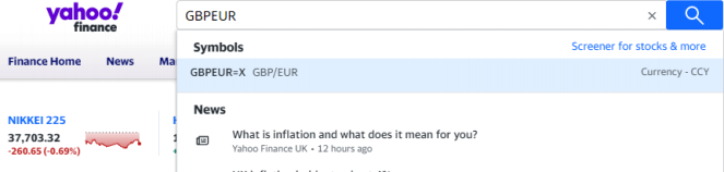
2.  Search for the exchange rate series you would like to study.  Suppose you are in- terested in GBP/EUR. You can type GBPEUR in the search box and then select GBPEUR=X.

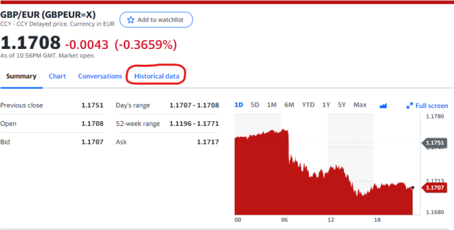
3. This brings you to the page for GBP/EUR with summary information displayed under the “Summary” tab. To access historical exchange rates, select the “Historical Data” tab.

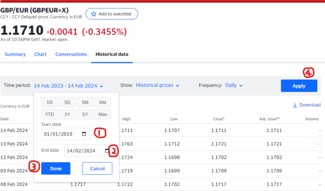
4.  Choose your time period, click done, and then click apply.

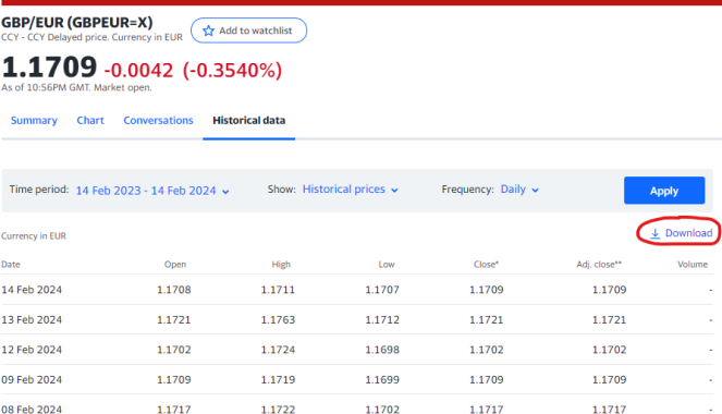
5.  Finally, click download and save the csv file to your computer.