Data Science & Machine Learning in Finance (ACCFIN5246) Assignment 2 – Spring 2024
Hello, dear friend, you can consult us at any time if you have any questions, add WeChat: daixieit
Data Science & Machine Learning in Finance (ACCFIN5246)
Assignment 2 – Spring 2024
Instruction
— This is an individual assessment. Answer all questions listed in Section 4: Q.1, Q.2, Q.3, Q.4.
— Submission to be made electronically via the course Moodle page.
— This submission includes a report including brief accounts on the logical steps taken, nu-merical answers, diagrams, and comments (each part in Section 4 specifies how answers are required to be presented).
— Submit only the main report (no additional spreadsheet, nor software routine, etc.).
— Clearly number each part in your report and structure the answers to follow the same order in Section 4: Q.1, Q.2, Q.3, Q.4. The project outline is presented across four sections to describe the implementations, estimation and arrangement of the results.
— Each part, within the assignment’s overall grade, carries a weight described below:
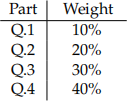
— Results should be reported in a clear format. Avoid reporting numbers in the ‘scientific format’ e.g. 7.2031e-06. All reported numbers should be rounded to two decimal points. For example, report 0.00 in place of 7.2031e-06.
— The project includes an Appendix (X1) which provides additional data and their descrip-tions.
Section 1: Models
Consider the standard and two extended capital asset pricing models characterised below in equa-tions (1)-(3), denoted as Model (A), Model (B) and Model (C), rspectively:
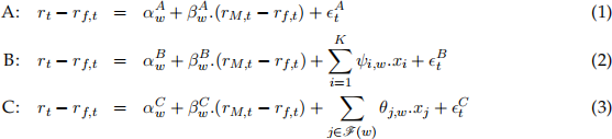
Each model aims at interrelating the real excess equity log-return as the outcome variable, on a given asset rt − rf,t where rf,t is the risk-free log-return, to the right-hand-side explanatory vari-ables, where:
[1.1] Time (daily frequency) is denoted by t = 1, . . . , T and the window index (consecutive days) is denoted by w = 1, . . . , W.
[1.2] Each x-covariate denotes an additional financial, market-level or macroeconomic variable, described in Appendix (X1).
[1.3] x-covariates are indexed by i and j in Model B and Model C, respectively, where i = 1, . . . , K and K describes the number of available covariates in Appendix (X1), whereas j ∈ F(w) refers to a sub-selection of all available covariates. The selected covariates included in set F(w) is carried out based on the learning method described in Section (3). Note that the selection outcome in F(w) is permitted to vary based on the rolling window.
[1.4] Specification error terms are denoted by  across Models A-C, respectively.
[1.5] Model constants and CAPM parameters are described by  and
and  , re-spectively, in Model A, Model B and Model C. The additional x-covariates are parameterised according to ψi,w and θj,w, in Model B and Model C, respectively.
The object of interest in each model is the time-varying coefficients described in [1.5]. Each model provides a suggested specification, ultimately aiming at uncovering the true but unobserved α and β.
Section 2: Data
The focus range covers 2000/01/03-2022/05/31, on a daily basis in Sheet (A) and separately on a monthly basis in Sheet (B). The dataset including the variables are provided on the course Moodle page, however additional data is required to be obtained:
[2.1] Observed Amazon Inc. daily stock price (variable AMZN) acquired from the Wharton Re-search platform (WRDS) for the construction of (rt) log-returns.
[2.2] Observed US daily equity market return (variable SP500) described by the S&P500 compos-ite market index return for the construction of (rM,t).
[2.3] The daily risk-free log rate (variable rf), associated with the US treasuries for the construc-tion of excess log-returns rt − rf,t and rM,t − rf,t (in real terms).
[2.4] Appendix (X1) provides the description of additional x-covariates.
[2.5] All prices in Sheet (A) have to be transformed into log-returns. All covariates in Sheet (B) to be used without any transformations.
[2.6] The eventual dataset including both Sheets (A) and (B) should be in a daily frequency. To this end, combine both sheets such that monthly frequency data in Sheet (B) are kept constant and repeated identically within each month versus varying other daily observations in Sheet (A).
[2.7] When there is a missing or non-numeric entry, remove the data for the specific day across all variables in the dataset.
Section 3: Implementations and Estimation Methodology
Implement a code to estimate all three models in equations (1)-(3), on a rolling window basis where w = 280. This indicates that windows include 280 consecutive (working) days as appear in the dataset and rolling forward by one day, amounts to a new window such that each two neigh-bouring windows overlap for 279 days. For each model, carry out the estimation as described below and store the specified results for w = 1, . . . , W:
[3.1] To estimate the parameter values described earlier for Model A, use the standard OLS method where only rt − rf,t and rM,t − rf,t are included. The estimation results produce  .
.
[3.2] To estimate the parameter values described earlier for Model B, use the standard OLS method where rt − rf,t and rM,t − rf,t are included, in addition to all of the x-covariates included in the Appendix (X1). The estimation results produce  .
.
[3.3] For estimation of the parameter values in Model C, use the Lasso regression method where rt−rf,t and rM,t−rf,t are considered in addition to all of the x-covariates included in the Ap-pendix (X1). The estimation method implements an additional learning parameter λw which determines the selection intensity (λ is characterised as the ‘cost’ associated with the Lasso constraint). Therefore the estimation results associated with the lasso regression produce 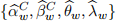 .
.
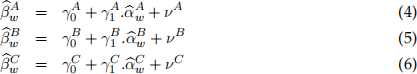
Once stored the three sets of estimation outpus: , , and , implement the following secondary regressions:
[3.4] Evaluate the following specifications and store the values for  ,
,  and
and  :
:
[3.5] Implement a forecasting framework to predict the one-step ahead value of the outcome vari-ables in equations (4)-(6). To carry out the prediction, use 14-consecutive window values ear-lier obtained: ,  , and
, and  within each model, to predict the next-step ahead outcome variable value and store the resulting forecast mean squared errors (FMSE) values for each of the expressions (4)-(6).
[3.6] Model A uses a minalistic approach without including any x-covariates, whereas Model C applies a learning-based method to select a sub-set of x-covariates. Consider an alternative extended specification in place of equation (4) based on  as input data in addition to x-covariates:

where the additional part incorporates the x-covariates now explicitly introduced to the specification, νD is the specification error term, the selection set is determined based on the Lasso approach and l denotes the index for selected x-covariates. This specification, first, is based on a minimalistic setup of Model A, leading to while, second, also in-forms the secondary regression in (7) through including the additional x-covariates. Note that the estimation is carried out only once and there is no further rolling window imple-mentations in equation (7). However, given that are already the outcomes of the rolling windows, you will need to set up the new dataset such that each pair  and
and  is considered together with the last value of the x-covariates. For instance, window 1 uses the original excess log-returns data from days 1 to 280, inclusive, leading to
  . Then the x-covariate values at day 280 are used to form the first row of dataset required for the estimation of expression (7). Similarly, window 2 uses the original data from days 2 to 281, inclusive, leading to
  . Then the x-covariates at day 281 are used to form the second row of the dataset required for expression (7), etc. This approach ensures that values for are paired with the most recent values from the x-covariate data, within each window w.
Section 4: Results and the Final Report
Your report should provide the numerical results and comments requested below. Please organise your report following the same structure arranged below by including the answers under parts [Q.1]-[Q.4].
[Q.1] Briefly explain the trade-offs associated between the model variance versus bias-squared to inform model selection. (Concise and less than 200 words) (Mark: 10%)
[Q.2] Report the estimated values for  and
and  in two separate overlaid dia-grams where the vertical axes show estimation values and the horizontal axes show window identifiers. (Mark: 20%)
[Q.3] Report the FMSE values associated with part [3.5]. Based on these values, provide com-ments which of the expressions (4)-(6) is considered most reliable to predict their outcome variables. (Concise and less than 200 words) (Mark: 30%)
[Q.4] Estimate the specification expressed in (7) based on the Lasso method. Report the estimated values for  and their p-values. Explain which of the expressions (6) or (7) is con-sidered more reliable to uncover the underlying relationship between the unobserved true α and β values. You may implement a FMSE measure to inform and test the prediction per-formance. Your comments are required to relate your conclusion to the methodologies and estimated values. (Concise and less than 350 words) (Mark: 40%)
2024-03-14