This assignment will be marked out of 100 marks and is worth 15% of the overall mark for the unit. Please check the unit outline for late penalties. This assignment is an individual assignment and is   not a group assignment. All work must be completed individually.

Please note that the screenshots included in this assignment specification may include previous years and dates. All dates in the text, and in the files provided in the data zip file, should be correct.

Submission

All submissions need to be electronic submissions through Canvas before the due date. You can submit multiple times, however only the latest version submitted on Canvas at the time of marking will be marked. Please note that you are able to submit after the due date has passed even if you have previous on-time submissions – this is to allow all students to submit late as per university policy.

Submission is to be one single zip file with a filename in the following format:

ITW-2024-S1-A1-YOURSTUDENTID.zip

Replacing YOURSTUDENTID with your student ID number.

This makes it easy for your marker to identify your submission once it has been downloaded from Canvas.

Which contains the following files:

1.    P1-YOURSTUDENTID-PaymentRequests.docx

2.    P1-YOURSTUDENTID-MailMerge.txt

3.    P1-YOURSTUDENTID-CanberraReport.docx

4.    P2-YOURSTUDENTID-SalesReports.xslx

As with the zip file name, replace YOURSTUDENTID with your student ID number. For example,a student with a Student ID of u123456 would submit a file named:

ITW-2024-S1-A1-u123456.zip

Which contains the following files:

1.    P1-u123456-PaymentRequests.docx

2.    P1-u123456-MailMerge.txt

3.    P1-u123456- CanberraReport.docx

4.    P2-u123456-SalesReports.xslx

Creating a zip file

The following instructions describe one way to create a zip file in Microsoft Windows. This has also been demonstrated in Lecture 2.

1.    Place all of your submission files into a single folder

2.    Right-click on the folder and select “Send to” and then “Compressed (zipped) folder” as shown in the screenshot below:

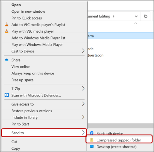
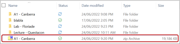
This will create a new Compressed (zipped) folder – as shown in the ‘Type’ column – which you can rename if required, and will contain a compressed copy of the folder you selected.

9.    Add a footer containing page numbers to all pages except the cover page. For even-

numbered pages, put the page number on the left; for odd-numbered pages, put the page

number on the right. Note that the cover page does not count for numbering nor for the

odd/even formatting. Therefore, the page where the table of contents starts on (which

should be page 2 in Word) should be numbered as Page 1 and have the number on the right- hand side.

10.  Resize the image provided in the Summary section so that it takes up no more than half the width and height of the page, place the image on the right-hand side of the page, and have  the text wraparound the image so there the text in the section is on the left-hand side of the page.

11.  Place the text provided below the image in the summary section in a text box, place the text box at the top of the image resized in the previous step.

12. Add a smart art diagram in the “Sister city and friendship city relationships” section where it is indicated, showing the information provided in an appropriate format. Remove the labels  (BEGIN SMARTART DIAGRAM, END SMARTART DIAGRAM).

13. Insert and resize following images inappropriate sections:

P1-Baptist Church.png and P1-Blundells' Cottage.png

14. Resize the images in the ‘ Development throughout 20th century” subsection so that it takes up no more than half the width and height of the page, place the images at appropriate places after applying appropriate text wraparound the images. Attribution of one of the images is missing! Add a text box below that image, and write the following information  inside the box:

Image by user: Adz

Creative Commons Attribution-ShareAlike 3.0

https://creativecommons.org/licenses/by-sa/3.0/

15. Change the references to footnotes. These references are clearly marked. Remove the labels (“FOOTNOTE:”).

16. Format the list in the “Ancestry and immigration” subsection appropriately. Remove the labels (BEGIN LIST, END LIST).

17. In the “Ancestry and immigration” subsection, change the information to the table appropriately. Remove the labels (BEGIN TABLE, END TABLE).

18. Format the bullet points in the “Infrastructure” section appropriately. Remove the labels (BEGIN BULLET POINTS, END BULLET POINTS).

19. Format all citations appropriately. Remove the labels (“CITATION:”)

20. Make sure the spelling is correct in the entire document (using Australian English spelling). 21. Generate the bibliography before the acknowledgment section.

22. Set the document properties as follows:

a.    Title: Canberra

b.    Subject: The Capital of Australia

c.    Author: your student ID number

d.    Manager: the unit convener’s name

e.    Company: Tourism Australia

f.     Category: Report

g.    Keywords: Canberra, history, demographic, infrastructure

Part 2 - Spreadsheet Editing (50 marks)

The exercises in Lab 2 – Spreadsheet Editing will provide good practice for this part of the assignment.

This part of the assignment places you in the role of a sales manager for a fictitious entertainment company. In this role, you are responsible for tracking and projecting sales and sales targets, and   tracking and managing the performance of sales staff.

For this part of the assignment, you will need the following files available in the P2Data folder in the AssignmentData.zip file that is available for download from Canvas:

1.    P2-Data1.xlsx

You will produce the following files which will contain your work for this part of the assignment and be part of the zip file which you will submit on Canvas (with YOURSTUDENTID replaced with your student ID number):

1.    P2-YOURSTUDENTID-SalesReports.xslx

Instructions

1.    Open P2-Data1.xlsx using Microsoft Excel. Use ‘Save As’ to save a copy of this file as P2-

YOURSTUDENTID-SalesReports.xlsx (replacing YOURSTUDENTID with your student ID

number). Make sure you save your work regularly to avoid losing any progress! The text and data that is included in P2-Data1.xlsx is the data you will be addingto and using for this part of the assignment.

2.    For all of the following steps, use a function wherever appropriate.

3.    For the Quarterly Sales Summary sheet, make the following additions:

a.    In the ‘Total 2021’ column (F), add formulas to calculate the total for sales across all four quarters for that type of network.

b.    In the ‘Projected 2022 Sales Increase’ column (G), add formulas to calculate the

projected 2022 sales increase which is the value in Total 2021 multiplied by the

Projected Sales Growth value in row 4. Complete the formula for ‘Classic Movie and TV Networks’ and use the fill option to copy the formula for the other types of network.

c.    In the ‘Totals’ row (12), add formulas to calculate the total for each quarter, total for 2021, and projected 2022 sales increase.

d.    In the ‘Trend’ column (H), add aSparkline to show the change in sales for each network over the quarters in 2021.

e.    Add a chart that shows how each of the networks contributed to the total 2021

sales. Make sure the chart has an appropriate title and labels. Place the chart below the table.

f.     In a cell directly below the chart, briefly (<200 words) justify your choice of chart type.

g.    Format the sheet appropriately, ensuring all cells and values are appropriately

formatted and the contents are entirely visible at 100% zoom. All sales figures are in dollars.

4.    For the Bonuses sheet, make the following additions:

a.    For the ‘Total Sales’ column (G), add formulas to calculate the total annual sales

(across all four quarters) of each sales representative’s sales. Apply appropriate conditional formatting to the total sales column so that the relative performance of each individual sales representatives compared to each other can be quickly seen.

b.    In the ‘Bonus’ column (H), add formulas so that sales representatives whose total

annual sales are above the average annual sales for all sales representatives receive a bonus (‘YES’), and the others do not (‘NO’). Also add conditional formatting in this column to highlight any ‘YES’ values.

c.    In the ‘Total’ row (18), add formulas to calculate the total sales by sales representatives for each quarter and across all four quarters.

d.    Under the Summary Statistics heading, for each entry enter formulas (in column D)  to calculate and display the statistics as listed. Note: You should not have to change the data table in order to accomplish this.

e.    Add a chart that shows how total sales by all sales representatives combined has

grown and shrunk across the four quarters. Make sure the chart has an appropriate title and labels. Place the chart below the table.

f.     In a cell directly below the chart, briefly (<200 words) justify your choice of chart type.

g.    Format the sheet appropriately, ensuring all cells and values are appropriately

formatted and the contents are entirely visible at 100% zoom. All sales figures are in dollars.

5.    For the Sales Projections sheet, make the following additions:

a.    In the ‘Total 2021’ column (B), change the static values to appropriate formulas that refer to the appropriate values in the Quarterly Sales Summary sheet. Also, add a

formula in the Totals row for this column (cell B12) to calculate the correct total.

b.    In the ‘% of Total Sales’ column (C), add the appropriate formulas to show the percentage contribution of each network’s sales to the total 2021 sales.

c.    In the ‘Target % of Target Total Sales’ column (F), add the appropriate formulas to

show the percentage contribution of each network’s target sales amount to the total target sales.

d.    Delete the target sales amount for International Networks (cell E11). Then use Goal   Seek to determine the target sale amount of International Networks that is required for it to makeup 13% of total sales coming from International Networks.

e.    Format the sheet appropriately, ensuring all cells and values are appropriately

formatted and the contents are entirely visible at 100% zoom. All sales figures are in dollars.

6.    Create a pivot table in a new sheet using all of the data (A9:G223) in the Trips sheet. Using this pivot table:

a.    What is the total of sales from trips for Film Entertainment Networks in Australia (AUS)? Enter this value in the cell A4 of the Trips sheet.

b.    How much did Lisa Vanderbeck spend on trips (Trip expenditures) in Quarter 3? Enter this value in the cell A5 of the Trips sheet.