Hello, dear friend, you can consult us at any time if you have any questions, add WeChat: daixieit

CMPUT 206 (LEC B1 Winter 2024): Assignment 4: Cell Segmentation | eClass

Opened: Saturday, 2 March 2024, 12:00 AM

Due: Friday, 15 March 2024, 11:59 PM

This assignment is worth 9% of the overall weight.

In this assignment

Part I (60%): we will be detecting cells in an image using blob detection techniques in Scikit-image.

Part II (40%): we will use watershed segmentation to find the boundaries of the cells we detected in part I.

You are provided with a single source file called A4_submission.py. You need to complete the functions and parts indicated in the source file. You can add any other functions or other code you want to use but they must all be in the same file. You need to submit only the completed A4_submission.py.

Part I (60%):

Start with the function part1() in A4_submission.py and nuclei.png

1. Create a Difference-of-Gaussian Volume (15%)

Create a 3-level Difference of Gaussian (DoG) volume by applying the given sigmas in the template A4_submission.py. Some instructions on how to calculate DoG are given in the comments.

The DoG filter can be implemented using skimage.filters.gaussian. You however CANNOT use skimage.filters.difference_of_gaussians.
All 3 levels of the volume must be stored in a single h × w × 3 numpy array where h and w are the height and width of the input image.

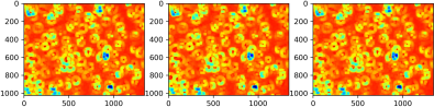
The output should look like this:

2. Obtain a rough estimate of blob center locations (30%)

Detect regional minima within the DoG volume.

As described here, regional minima are defined as "connected components of pixels with a constant intensity value, and

whose external boundary pixels all have a higher value".

To perform this, you can use the scipy function scipy.ndimage.filters.minimum_filter.

The output of this step using scipy.ndimage.filters.minimum_filter will also be of size h × w × 3.

The detected minima depend heavily on the parameters used for defining the region size. For instance, if the scipy function is used, then its second argument "size" must be chosen carefully.

It should also be noted that the scipy function returns the actual values of the detected minima rather than their locations so additional steps will be needed to convert its output to the required binary image. The binary image will be of the same size as the DoG volume that contains 1 at locations of the regional minima and 0 everywhere else.

Collapse this 3D binary image into a single channel image by computing the sum of corresponding pixels in the 3 channels. This can be done using np.sum.

Show the locations of all non-zero entries in this collapsed array overlaid on the input image as red points.

The locations of non-zero entries can be found using np.nonzero while the plotting can be done using plt.scatter. All code for plotting has been provided in the template.

The outputs should look like this:

The output after finding regional minimas using scipy.ndimage.filters.minimum_filter:

The output of rough blob centers detected:

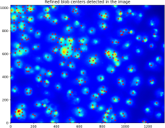
3. Refine the blobs using Li thresholding(15%)

Apply Gaussian filtering usingskimage.filters.gaussian with a suitably chosen sigma.

Convert the blurred image to 8-bit unsigned integer format using skimage.img_as_ubyte. (These first two steps have already been done for you in the template code)

Apply Li thresholding on the blurred image using skimage.filters.threshold_li to obtain the optimal threshold for this image.

Remove all minima in the output image of "Obtain a rough estimate of blob center locations" where pixel values are less than the obtained threshold

Show the remaining minima locations overlaid on the input image as red points.

The output should look like this:

Part II (40%):

Implement Minimum Following watershed segmentation to find the boundaries of the cells we detected in part I.

Code you need to complete for this part: The three functions getRegionalMinima(img), iterativeMinFollowing(img, markers) and is_4connected(row, col, row_id, col_id). You will need to call the getSmallestNeighborIndex (img, row, col) function in getRegionalMinima(img) and iterativeMinFollowing(img, markers). Please do not modify code under part2().

The function getSmallestNeighborIndex (img, row, col) has been given in your code template. It returns the location of the smallest 4-connected neighbor of the pixel at location [row,col]. Within getSmallestNeighborIndex (img, row, col), there is a function call to is_4connected(row, col, row_id, col_id). This function checks for 4-neighborhood connectivity. 4-connected neighbors here refer to the horizontal and vertical pixel neighbors. Itʼs illustrated below. You are first required to finish is_4connected(row, col, row_id, col_id) so that your getSmallestNeighborIndex (img, row, col) works as expected.

1. getRegionalMinima(img) : This function computes the local minima in the given image by comparing each pixel in the image to its 4-connected neighbours and marking it as a local minimum if its value is smaller than or equal to all of them.

The output of this function is a 32-bit integral image that contains non-zero labels for all local minima pixels and zero everywhere else

This function is used to generate markers for the next function iterativeMinFollowing(img, markers).

2. iterativeMinFollowing(img, markers): This function uses the minimum following algorithm to label the unlabeled pixels in the marker image generated by the previous function.

The steps described in the lecture notes are difficult to implement without recursion so you will instead be implementing an iterative variant of this algorithm that performs multiple passes over the image. At the beginning of each pass, set a counter (n_unmarked_pix) to zero. In each pass, the entire image is traversed pixel by pixel, and the following steps are performed for each pixel location (i, j) :

If (i, j)is already labeled (i.e. it has a non-zero value), leave it unchanged

Else, find the pixel location with the smallest intensity value in the 4 connected neighborhoods of (i, j). Refer to this location as (m, n).

If (m, n) has a nonzero label, copy this label to that of (i, j)

If the label of (i, j) is still 0, increase the counter by 1.

The counter, which represents the number of unlabeled pixels, should decrease in each iteration. Print this counter after each iteration. Stop the iteration when the counter is 0 because at this point all the pixels have been labeled. If the counter does not decrease, then there must be a bug in either this function or in getRegionalMinima that was used for generating the markers.

iterativeMinFollowing(img, markers) should return the final labeled image which must also be in a 32-bit integral format like the input markers. You should not modify the contents of the markers directly - first, make a copy and then write any changes there.

To test whether all your functions are working properly, a test case A4_test_image.txt is provided. The code for executing the test case has already been added to your code template. This code prints both the initial markers generated by getRegionalMinima and the final labeled matrix produced by iterativeMinFollowing. There is also a test case to make sure your getSmallestNeighborIndex (img, row, col) is working as expected.

The outputs for the test cases should look like this:

Test image:

Testing function getSmallestNeighborIndex...

Location of the smallest 4-connected neighbor of pixel at location [0,0] with intensity value 10.0: [1, 0] with value 75.0

Testing function getRegionalMinima...

markers:

Testing function iterativeMinFollowing...

labels after iteration 1:

n_unmarked_pix: 5

labels after iteration 2:

n_unmarked_pix: 1

labels after iteration 3:

n_unmarked_pix: 0

All pixels have been labeled! Stop iteration.

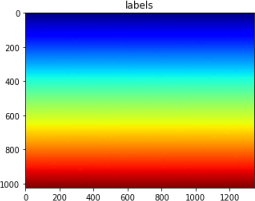
Final labels:

Note!!!: The output for the test case of iterativeMinFollowing above shows/prints the marked labels after each iteration. This is just for your reference on how iterativeMinFollowing is supposed to work. However, you simply only need to print n_unmarked_pix for each iteration and the final labels.

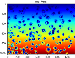
Image reconstruct and draw their boundaries

The imreconstruct (marker,mask) function performs morphological reconstruction of the image marker under the image mask and returns the reconstruction in imreconstruct. The elements of the marker must be less than or equal to the corresponding elements of the mask. If the values in the marker are greater than the corresponding elements in the mask, then imreconstruct clips the values to the mask level before starting the procedure. The function imimposemin(marker,mask) can revise the image to minimize pixel values in some regions.

Both imreconstruct (marker,mask) and imimposemin(marker,mask) have been provided in the template and should not be edited.

The outputs of part2 should look like this: