闪电代写 -代写CS作业_CS代写_Finance代写_Economic代写_Statistics代写_代码代做_IT代写_加急帮助

Hello, dear friend, you can consult us at any time if you have any questions, add WeChat: daixieit

Nonlinear econometrics for inance

HOMEWORK 1

(Review of linear econometrics and review of methods)

Problem 1 (Linear econometrics.) (60 points) Household inance is a growing ield in inance. In this homework you will study medical household expenditures, using data from a developing region in Vietnam. The dataset in the ile vietnam. csv contains the following information:

. sex: gender of household head (male, female)

. age: age of household head

. education: years of schooling of household head

. farm: does the household engage in farming?

. urban: is the household in an urban area?

. hhsize: number of people in the household

. totalexp: household total expenditure

. medexp: household medical expenditure

. community: community where the household lives

Given this information, you need to perform linear regression in Python to understand the drivers of medical expenditures.

(1) (3 points) Generate an histogram of the medical expenditures and com- pute descriptive statistics (mean, median, standard deviation, mini- mum, maximum). Is the distribution symmetric? Provide an economic justiication for your answer: what could explain the lack (or presence) of symmetry?

(2) (3 points) Take a logarithmic transformation of the medical expendi- tures. Now, plot the histogram of the log-expenditure. What do you notice? How would you explain the change?

Begin by excluding all categorical variables (sex, farm, urban and commu- nity).

(3) (6 points) Transform total expenditure into logarithms and run a re- gression of the log medical expenditures on the non-categorical ex- planatory variables (with total expenditures in log). The model you are estimating is:

log(medexpi ) = θ0 + θ1 agei + θ2 educationi + θ3 hhsizei + θ4 log(totalexpi ) + εi ,

where εi is an error term and i corresponds to a speciic household. Report the results of the regression in a table. At a minimum, your table should contain the estimated parameters, the standard errors, the t-statistics and the p-values for the standard tests of the hypothesis that the parameters are equal to zero.

Please note: You should construct all of the quantities from scratch using their defnition from linear econometrics. The same observation applies to all other questions below. You can use a Python regression function only to check your results.

(4) (3 points) What does the model say about the determinants of (log) medical expenditures? You should comment on the sign, statistical and economic signiicance of the estimated coefficients.

(5) (3 points) In a regression - without log transformations - of y on x the regression coefficient measures Δy/Δx. What is the interpretation of θ 1 here? Hint: you are regressing a log variable (log(medexpi )) on a variable that is not in logs (agei ).

(6) (3 points) What is the interpretation of θ4 ? Hint: you are regressing a log variable (log(medexpi )) on another log variable (log(totalexpi )).

(7) (4 points) We want to test whether the coefficient θ4 for log(totalexp) is statistically signiicant. Test the hypothesis using the relevant test statistic. Does log(totalexp) have more or less explanatory power than age?

(8) (3 points) We want to test whether the coefficient θ4 for log(totalexp) is statistically signiicant. Test the hypothesis using the relevant p-value.

(9) (5 points) Test the single linear restriction θ2 = -5θ1 using the relevant test statistic.

(10) (3 points) Test the single linear restriction θ2 = -5θ1 using the relevant p-value.

(11) (5 points) Test the multiple linear restriction θ2 = -0.05 and θ3 = 0.05 using the relevant test statistic.

(12) (3 points) Test the multiple linear restriction θ2 = -0.05 and θ3 = 0.05 using the relevant p-value.

(13) (4 points) Using the estimated model, predict medical costs for a house- hold whose head is 36 years old, has 10 years of education, the house- hold size is 4 and the total logarithm of expenditures is 10. Is the prediction lower or higher than the mean of the distribution of the medical expenses? (Recall that the regression gives you a prediction for the log of the medical costs (say, log(y)) not for the medical costs (say, y). Hence, after you fnd the prediction for the log of the medical costs, you need to make a transformation to fnd a prediction for the medical costs themselves. Hint: if log(y) is normal, y is lognormal. What is E(y) for a log normal random variable? )

Now, take the categorical variables (excluding “community”, which you should ignore) into account using dummy variables (https://en.wikipedia.org/wiki/Dummy_variable_(statistics)). Re-run the regression using the cat-egorical variables.

(14) (3 points) Which dummies are statistically signiicant?

(15) (3 points) How much more (or less) do households with males heads spend relative to households led by female heads (controlling for all other variables)?

(16) (3 points) How much more (or less) do farming households spend rela- tive to non farming households (controlling for all other variables)?

(17) (3 points) Using your model, predict medical expenses for anon-farming, urban household whose head is a 43 years old male with 10 years of education, in which there are 3 people and total expenditure is 45,000.

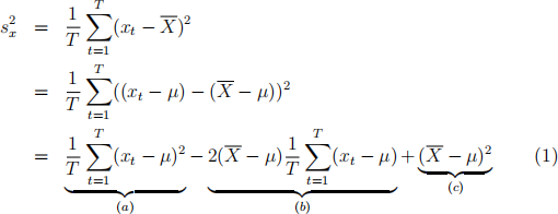
Problem 2 (Review of methods). (30 points) Assume an iid sample {x1 , x2 , ..., xTg from some distribution with expected value μ and variance σ2 . A natural estimator for the true variance (i.e., σ 2 ) of the random variable

which generates the data is the sample variance, namely = T/1(xt - )2 , where deines the sample mean, i.e., T/1 xt.

First, let us focus on the inite-T (or inite-sample) properties of :

(1) (4 points) Show that the sample variance is biased for the true variance σ2.

(2) (3 points) How would you correct the bias?

(3) (3 points) What is the bias of the infeasible variance estimator ,inf = T/1(xt − µ) 2 . Why am I calling this estimator infeasible?

Now, let us turn to the large-T (or ininite-sample or asymptotic) properties of . Write the following:

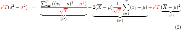
Now, subtract from the left-hand side and from the right-hand side of Eq. (1) and standardize by to obtain:

(4) (4 points) Show that is consistent for σ2 by applying the LLN to (a), (b) and (c) in Eq (1).

(5) (4 points) Show that ( − ) is asymptotically normal by ap-plying the LLN, the CLT and Slutsky’s theorem to (a*), (b*) and (c*) in Eq. (2).

Notice that consistency is a statement about sample averages, like , con-verging (as T → ∞) to expected values. Asymptotic normality is a statement about demeaned (by , in our example) and standardized (by , in our example) sample averages, like ( − ), converging (as T → ∞) to a mean-zero normal distribution.

(6) (6 points) Use my sample Python codes from Lecture 1 to write a code which shows consistency of . You should draw your observations from a random variable which is neither exponential nor normal.

(7) (6 points) Use my sample Python codes from Lecture 1 to write a code which shows asymptotic normality of ( − ). You should draw your observations from a random variable which is neither exponential nor normal.