Math 466 Assignment 7, The Linear Quadratic Regulator, Spring 2024
Hello, dear friend, you can consult us at any time if you have any questions, add WeChat: daixieit
Math 466 Assignment 7, The Linear Quadratic
Regulator, Spring 2024
Due: Monday, March 4th
February 25, 2024
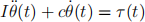
In this assignment we design and simulate a full state feedback LQR control law for a rotating antenna. The motion of the antenna can be described by the linear second order non-homogeneous differential equation given by
with initial conditions

where I is the effective moment of inertia of all the rotating parts including the antenna, c ≥ 0 is the coefficient of viscous (i.e. air; the antenna is in low earth atmosphere, not the vacuum of space) friction, τ (t) is the torque applied by the motor that effects the rotation at time t ≥ 0, and θ(t) is the angular position of the antenna at time t ≥ 0. (The basis for the model is simply Newton’s second law, F = ma, in the context of rotary motion, i.e. torque equals the moment of inertia times the angular acceleration. The friction term is modeled as a torque that is proportional to the velocity so that it is in the direction opposite to the motion of the antenna.) The motor torque at time t ≥ 0 is assumed to be proportional to u(t), the input voltage to the motor, with constant of proportionality b > 0. In your calculations below use the following values:  ,and I = 10kgm2. The output variable is the angular position and the angular velocity of the antenna.
Problem 1. Rewrite the model as a first order system of the form
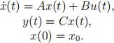
What are the matrices A, B, C, and x0?
Problem 2. Assume zero-order hold inputs with a time sampling interval of length τ = 0.1s (i.e. 10 Hz), that is, u(t) = uj , t ∈ [jτ,(j + 1)τ ), j = 0, 1, 2, ..., and rewrite the model found in Problem 1 above as a discrete time system of the form
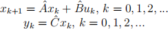
What are the matrices  ,
,  , and
, and  ?
?
Problem 3. Use the LQR theory derived in class to determine a full state feedback control law that minimizes the performance index

where α ≥ 0, β ≥ 0, ρ > 0, γ ≥ 0, δ ≥ 0 and k1 a positive integer, are design parameters.
Problem 4. Use Simulink to construct a simulation of the closed loop system. Assume an initial angular position of θ0 = 0.1rad and an initial angular velocity of θ1 = 0. Include scopes and output variables that display and collect θ(kτ ),  (kτ ), uk, the feedback gain Kk,
 , where
  is the optimal controller.
Problem 5. Run your simulation for different values of the design parameters, analyze the results and produce a report detailing your findings which includes appropriate plots and tables. Be certain to compare the closed loop performance of the system with the open loop performance (i.e with no control).
Problem 6. Show (theoretically) that the Riccati matrices, Pk, k = 0, 1, ..., k1 are all posi-tive semi-definite and symmetric.
Problem 7. Re-derive the solution to the LQR control problem as was done in class, but this time assume that the matrices A = Ak, B = Bk, and C = Ck and the weights α = αk, β = βk, and ρ = ρk are all time dependent. What assumptions if any do you require?
Problem 8. Redo Problems 1 -5 but this time assume that you only want to penalize (or drive to zero) the angular position and do not care about the angular velocity. However, assume that you are able to observe or measure both the angular position and the angular velocity.
2024-03-06