MATH 308 Midterm Project
Hello, dear friend, you can consult us at any time if you have any questions, add WeChat: daixieit
MATH 308
February 18, 2024
Midterm Project
• This midterm project is due on March 10 at 11:11pm.
• You can work in groups of up to 2 people.
• Datasets can be downloaded from MyCourses.
• Please submit your solutions as pdf files via Crowdmark. Make sure to upload a separate pdf file containing your entire code with proper comments about the purpose of each code chunk.
1 SVD for learning word embeddings
This question is about word embeddings. A word embedding is a mapping from words, to vector representations of the words. Ideally, the geometry of the vectors will capture the semantic and syntactic meaning of the words—for example, words similar in meaning should have representations which are close to each other in the vector space. A good word embedding provides a means for mapping text into vectors, from which you can then apply all the usual learning algorithms that take, as input, a set of vectors. Word embeddings have taken NLP by storm in the past 5-10 years, and have become the backbone for numerous NLP tasks such as question answering and machine translation. There are neural-network approaches to learning word embeddings, but in this question we will study a simple SVD based scheme which does a surprisingly good job at learning word embeddings.
We have created a word co-occurrence matrix M of the 10,000 most frequent words from a Wikipedia corpus with 1.5 billion words. Entry Mij of the matrix denotes the number of times in the corpus that the ith and jth words occur within 5 words of each other. [Note–the values are not all integers, since we weighted the co-occurrences by the distance—co-occurrences at distance 5 are weighted less than cooccurrences at distance 2 or 3.] The file co_occur.csv contains the symmetric co-occurence matrix, M. The file dictionary.txt contains the dictionary for inter-preting this matrix, the ith row of the dictionary is the word corresponding to the ith row and column of M. The dictionary is sorted according to the word frequencies. Therefore the first word in the dictionary—“the” is the most common word in the corpus and the first row and column of M contains the co-occurrence counts of “the” with every other word in the dictionary.
1. Make sure you can import the given datasets into R or Python you’re using. Also, make sure you can interpret the entries of the co-occurrence matrix using the dictionary, you can try to find the co-occurrence of a few pairs of common words to make sure of this.
2. Let matrix M denote the 10000 × 10000 matrix of word co-occurrences. In light of the power law distribution of word occurrences, it is more suitable to work with the normalized matrix ˜M such that each entry ˜Mij = log(1+Mij ). For the remainder of this problem, we will work with this scaled matrix, ˜M. Compute the rank-100 approximation of ˜M by computing the SVD ˜M = UΣV > . Plot the singular values of ˜M. Does ˜M seem to be close to a low rank matrix? [Hint: Computing the full SVD would take a bit of time—instead you should compute just the top 100 singular values/vectors and save this decomposition rather than recomputing every time you work on this project!]
3. Note that as the matrix ˜M is symmetric, the left and right singular vectors are the same, up to flipping signs of some columns. We will now interpret the singular vectors (columns of U or V ). For any i, denote vi as the singular vec-tor corresponding to the ith largest singular value. Note that the coordinates of this vector correspond to the 10,000 words in our dictionary. For a given vector vi , you can see which words are most relevant for that vector by looking at the words corresponding to the coordinates of vi that have the largest pos-itive, and largest negative values. This allows you to get a rough sense for the semantic information that is captured in each of the singular vectors. Find 5 interesting/interpretable singular vectors, and describe what semantic or syn-tactic structures they capture. For each of the 5 vectors you choose, provide a list of the 10 words corresponding to the coordinates with the largest positive values and the 10 words corresponding to the coordinates of that vector with the most negative values. Not all of the singular vectors have easy-to-interpret semantics; why would you expect this to be the case?
4. Let V denote the 10000 × 100 matrix corresponding to the top 100 singular vectors. Normalize the rows of V such that each row has unit ` 2 norm. We will regard the ith row of V as the (100-dimensional) embedding of the ith word. We will now explore a curious property of these word embedding—that certain directions in the embedded space correspond to specific syntactic or semantic concepts. Let V1 ∈ R 100 be the word embedding for “woman” and V2 ∈ R 100 be the word embedding for “man”. Let V = V1 − V2.
(a) Project the embeddings of the following words onto V : boy, girl, brother, sister, king, queen, he, she, john, mary, wall, tree. Present a plot of pro-jections of the embeddings of these words marked on a line. For example, if the projection of the embedding for “girl” onto V is 0.1, then you should label 0.1 on the line with “girl”. What do you observe?
(b) Present a similar plot of the projections of the embeddings of the following words onto v: math, matrix, history, nurse, doctor, pilot, teacher, engi-neer, science, arts, literature, bob, alice. What do you observe? Why do you think this is the case? Do you see a potential problem with this? (For example, suppose LinkedIn used such word embeddings to extract infor-mation from candidates’ resumes to improve their “search for qualified job candidates” option. What might be the result of this?)
(c) Propose one method of mitigating the problem discussed in the previous part. There are many acceptable answers, and this is an ongoing area of research, so be creative and do not worry about making your answer overly rigorous. [Hint: If you need inspiration, see the original paper that surfaced this issue and discussed some approaches to “debiasing” word embeddings.]
5. In this question we will explore in more depth the property that directions in the embedded space correspond to semantic or syntactic concepts.
(a) First, we will define a similarity metric for words: the similarity of two words will be defined as the cosine-similarity between their embeddings.
As all the word embedding vectors have unit ` 2 norm, i.e. k Vik 2 = 1, the cosine similarity between two words i and j with embeddings Vi and Vj is equal to the inner product V1 > V2. Now that we have a similarity metric defined, we can have some fun with these embeddings by querying for the closest word to any word we like! Using this definition of similarity, what are the most similar words to “montreal”?
(b) Because word embeddings capture semantic and syntactic concepts, they can be used to solve word analogy tasks. For example, consider an analogy question— “man is to woman as king is to ? ”, where the goal is to fill in the ”?”. This can be solved by finding the word whose embedding is closest to Vwoman − Vman + Vking in cosine similarity. You can do this by a nearest neighbor search across the entire dictionary—excluding the three words man, woman, king which already appear in the analogy as they cannot be valid answers to the question. Here Vi ∈ R 100 represents the word em-bedding for the word i. We have provided a dataset, analogy_task.txt, which tests the ability of word embeddings to answer analogy questions. Using the cosine similarity metric, find and report the accuracy of the word embedding approach to solving the analogy task. Comment on the results–which analogies seemed especially difficult for this approach? Give 3 examples of “difficult” analogies that were solved incorrectly, and explain why those analogies might be difficult. (Ideally, for your three examples the correct answer wouldn’t even be in the top 5 guesses of this approach.)
(c) (Bonus) Your goal is to now improve the score of the word embeddings on the analogy task. Feel free to try any alternative scheme for learning word embeddings, but using only the cooccurrence matrix we have provided. Discuss the approaches you tried, what informed the choices, and the results they obtained. Showing that certain approaches obtain a poor accuracy is also valuable too. Your score will be based on a combination of the discussion and the best accuracy you obtain.
Deliverables:
Discussions for part 2, 3, 4, 5. Plot for part 2, 4. Provide code for all parts in the appendix as a separate PDF file.
2 SVD for image compression
Download p5_image.gif. It is a 1600 × 1170, black and white drawing of Alice conversing with a Cheshire Cat. We will think of this image as a 1600 × 1170 matrix, with each black pixel represented as a 0, and each white pixel represented as a 1. We will observe this matrix under various approximations induced by its SVD.
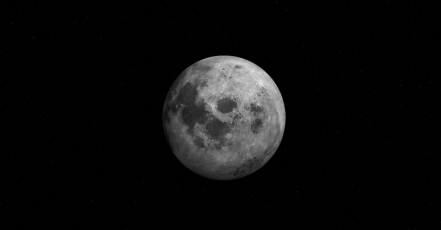
1. Before running SVD on Alice, think about what you expect the rank 1 ap-proximation given by SVD to look like. To guide your thinking, consider the following simpler picture, where black pixels have value 0. Qualitatively de-scribe the rank 1 approximation (given by SVD) of the following picture of the moon. Explain your reasoning. [Hint: it might be helpful for you to sketch what you expect the answer to be—and make sure it is rank 1!]
2. Run SVD and recover the rank k approximation for the image of Alice, for k ∈ {1, 3, 10, 20, 50, 100, 150, 200, 400, 800, 1170}. In your assignment, include the recovered drawing for k = 150. Note that the recovered drawing will have pixel values outside of the range [0, 1]; feel free to either scale things so that the smallest value in the matrix is black and the largest is white, or to clip values to lie between 0 and 1.
3. Why did we stop at 1170?
4. How much memory is required to efficiently store the rank 150 approximation? Assume each floating point number takes 1 unit of memory, and don’t store unnecessary blocks of 0s. How much better is this than naively saving the image as a matrix of pixel values?
5. Details of the drawing are visible even at relatively low k, but the gray haze / random background noise persists till almost the very end (you might need to squint to see it at k = 800). Why is this the case? [For credit, you need to explain the presence of the haze and say more than just ”the truncated SVD is an approximation of the original image.”]
Deliverables:
Discussions for part 1, 2, 3, 4, 5. Plot for part 2. Provide code for all parts in the appendix as a separate PDF file.
2024-03-06