BME 514 Spring 2024 LAB 3: LINEAR & NONLINEAR ANALYSES OF HEART RATE VARIABILITY
Hello, dear friend, you can consult us at any time if you have any questions, add WeChat: daixieit
BME 514
Spring 2024
LAB 3: LINEAR & NONLINEAR ANALYSES OF HEART RATE VARIABILITY
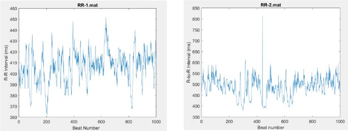
In this assignment, you will be given two datasets: RR-1.mat and RR-2.mat. Each of these datasets contains the RR-interval time-series determined from the electrocardiograms (ECG) of two-week old sleeping infants. RR-2.mat is measured from a baby with prenatal exposure (through the mother) to cocaine, whereas RR- 1.mat is from a normal control. Your task is to employ linear and non-linear time-series analyses to detect the differences (if any) in dynamics between these two datasets. In a real-world application, we would, of course, need to derive conclusions based on many datasets in each group – but since this is just a class assignment, the idea is to give you a sense of what this kind of analysis entails.
Each RR time series was constructed in the following way. From the ECG signal, the R-waves were first identified. Then, the times between successive R-waves (RR intervals, in milliseconds) were calculated. Thus, each RR value is separated from its predecessor and successor by one beat. Beat-to-beat plots of RR- 1 and RR-2 are displayed below:
Questions to be addressed:
(a) First, it is always useful to plot your data and to inspect them visually. Plot both datasets using the same scales on both sets of axes to facilitate comparison. The RR values are given in milliseconds. The time scale (horizontal axis) should be in number of beats.
(b) Present Poincare plots for each of the RR datasets: ie. plot RR at beat n+1 versus RR at beat n. By visual examination of the Poincare plots, comment on the similarities and differences that you notice between the two subjects
(c) Next, compute the power spectra of these 2 datasets using the periodogram method. However, in order to do this, you would first need to resample each dataset with a uniform sampling rate, since they have been given to you on a beat-by-beat basis. Let us select a sampling rate of 4 Hz. Briefly describe how you have chosen to convert the beat-by-beat data into a uniformly sampled time-series. Subsequently, remove the mean and linear trend from each of the resampled datasets before you compute their power spectra. To facilitate comparison, use the same scales for the horizontal and vertical axes of your plots. Deduce the contribution (in %) of the “low-frequency” (0.03 - 0.3 Hz) and “high-frequency” (0.3 - 2 Hz) bands to the total power (ie. the variance) of each dataset. Briefly comment on the similarities and differences between the two datasets.
(d) Use the Matlab program (sampen.m) provided in Blackboard to calculate the sample entropy (SampEn) for each beat-to-beat dataset. (Before applying this program to the datasets, it would be useful to test it program out on known test signals – eg. a sinusoidal waveform (SampEn low) and a Gaussian white noise sequence (SampEn high).
(e) Use the method of surrogate data to determine the extent to which the dynamics of each dataset are nonlinear:
(1) Generate 10 sets of surrogate data for each original dataset by randomizing the phases
of the original Fourier transform (FT) and computing the inverse FT. These 10 surrogate sets should have the same power spectrum as the original time-series, and thus have the same linear correlation structure. See the appendix to this assignment sheet for details on how to generate surrogate data. For the sake of simplicity, we will skip the “amplitude
adjustment” part of this surrogate data generation procedure – I will elaborate in class.
(2) Compute the SampEn value for each of the surrogate data sets. From the 10 SampEn values for the surrogate data, compute the mean and standard deviation. Assuming the distribution of these SampEn values to be Gaussian, the 95% confidence limits for the linear process underlying these surrogate data can be determined by assuming these bounds to lie ± 2 standard deviations from the mean surrogate SampEn value. Compare the SampEn of the original (true) dataset with the 95% confidence limits of the surrogate SampEn values. The further the former is from the 95% range of surrogate SampEn values, the more nonlinear the underlying dynamics. On the other hand, if the SampEn of the true dataset lies within the 95% confidence limits of the surrogate SampEn values, we must conclude that any nonlinearity in the underlying process is undetectable. Perform this test on both the normal and cocaine datasets.
(f) Briefly summarize the conclusions of this study. For instance: Which dataset has more low- frequency (0.03 - 0.3 Hz) vs. high-frequency (0.3 - 2 Hz) content? Which dataset is more "irregular" than the other? Which dataset would you consider to be more "nonlinear" in dynamics?
DUE DATE FOR LAB 3: TUESDAY 3/5 @ 11:59pm
APPENDIX 1: GENERATION OF SURROGATE DATA
Your program should follow these steps:
1. Read in the time series.
2. Take the Fourier transform of your data. You now have an array of complex numbers.
3. Set the seed of the random number generator to a value you specify.
4. For each of the complex numbers in (2), except for the first FFT value (corresponding to zero frequency) and the FFT value corresponding to the Nyquist frequency (ie. 1/2 the sampling frequency), do the following:
• Calculate r, the absolute magnitude of each FFT value.
• Generate a random number θ uniformly distributed between zero and 2π .
Most computer random number generators create a number that is uniformly distributed between zero and one, so all you need to do is multiply the output of the random number generator by 2π .
• Replace the real part of each FFT value by r cos θ and the imaginary part by r sin θ . Many Fourier transform routines perform calculations for both positive and negative frequencies. If this is the case for you, then at any given frequency you will generate only one θ at each frequency, using θ for the positive frequency and -θ for the negative frequency. (When taking the Fourier transform of a real time series, the result at frequency -ω is the complex conjugate of the result at ω.)
Leave the FFT values corresponding to the zero (DC) and Nyquist frequencies alone.
5. Take the inverse Fourier transform of the phase-randomized data you generated in (4).
6. Check the real parts of the inverse FFTs in (5). If you have done things correctly, the numbers should all be real, except perhaps for a tiny imaginary component due to computer round-off error. In order to produce a different realization of the surrogate data, change the random seed that was set in step (3).
In practice, a number of mistakes can be made. The most common is to forget to use the same θ for corresponding positive and negative frequencies. If you find that, after taking the inverse
Fourier transform, the imaginary part of the answer is not negligible, then you have probably made this mistake.
To test your program, generate a sine wave that has an integer number of cycles. For example,
if you have N points in your time series, then sin(2πt 10/N) for t = 1,..., N will have 10 cycles. The surrogate data generated from this sine wave should have exactly the same number of cycles, and be shifted only in phase. If you make a sine wave with a non-integer number of cycles (say, 10.5), then you will notice that the surrogate data looks like a sine wave whose amplitude slowly changes.
Make a long random time series that consists of zeros and ones. The surrogate data generated from this time series will have the same autocorrelation function, but will not be zeros and ones.
The amplitudes in the surrogate data will have a Gaussian distribution.
2024-03-05