Hello, dear friend, you can consult us at any time if you have any questions, add WeChat: daixieit

AD685 - MIDTERM EXAM

Spring 2020

Problem 1. Data were collected from a random sample of 220 home sales from a community in 2013. Let Price = selling price (in $1000), BDR = number of bedrooms, Bath = number of bathrooms, Hsize = size of the house (in square feet), Lsize = lot size (in square feet), Age = age of the house (in years), and Poor = binary variable that is “1” if the condition of the house is reported as poor, and is 0 otherwise. An estimated regression yields:

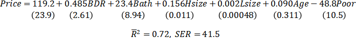
Number in parentheses below each estimated coefficient is the estimated std err (coefficient)

a. (10 pts) What is the predicted price of a house that has 4 BDR, 3 Bath, has 3,000 sq ft of living quarters, a lot size of 5,000 sq ft., it is 5 years old and is in good condition? What would be the price of this house if it were 4 years old and in poor condition?

b. (10 pts) Construct a 95% confidence interval (standard normal critical value) for the slopes of BDR and Bath, individually, and check whether they are statistically significant.

c. (20 pts) A colleague of yours posits that the slope on Hsize is “0.10” and that the slope on the Poor indicator is “-40”. Calculate the t-statistics and their p-values (round the t-stats to 2 decimals and use the std normal table) You must calculate the p-values in order to test at 10% significance whether your colleague is right.

Problem 2. You are considering the risk-return profile of some “Equity Mutual Fund” for investment. The Equity fund promises an expected return of 7% with a standard deviation of 10%. Assume that the returns are normally distributed.

a. (9 pts) Find the probability of earning a return between 2% and 22% for the Equity fund.

b. (6 pts) Find the probability of earning a return less than “-1%” for the Equity fund.

Note: You may round transformed Z-values to 2 decimals to make it easier to look at the table, but show all the decimals for the probability in the normal table.

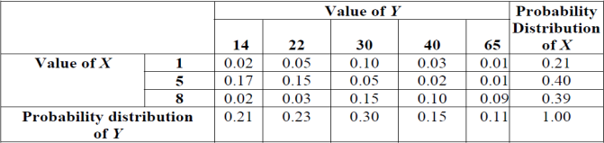
Problem 3. The following table gives you the probability distribution of X (last column) and Y (last row) as well as the joint probability distribution of X and Y (inner matrix of 3x5 elements).

a. (7 pts) Find the mean and std dev of Y

b. (8 pts) Find the conditional mean and conditional std dev of Y given that X=8.

Problem 4

The table of estimated regressions of the average of the reading and math scores on the Stanford 9 Achievement Test uses data for 1999 from all K–6 and K–8 districts in California. The variable of interest is the student-teacher ratio. N= 464 observations in each regression

a. (5 pts) What can you say about the relevance of the variable of interest X1 across regressions?

b. (5 pts) Does the regression fit improve when we add control variables to X1? Explain briefly

c. (10 pts) Discuss briefly the R2 and SER obtained in regression of column (2).

d. (10 pts) Construct the homoskedasticity-only F-statistic for testing β2=β3=β4=0 in regression #5. Use the 5% significance asymptotic CV = 3.0. Are the control variables jointly significant?