PPHA 421 Problem Set 3 Winter 2024
Hello, dear friend, you can consult us at any time if you have any questions, add WeChat: daixieit
PPHA 421
Problem Set 3
Winter 2024
Due date: Thursday, February 22 at 11:59 PM. You must submit via Gradescope on Canvas. Answers must be typed. No late problem sets will be accepted.
Group work: You may work in groups of up to three on your problem sets, but you must turn in your own problem set, with answers written in your own words. You may share code with other members of your group, but you may not share written answers with other students (including members of your own group).
Code: All coding in problem sets must be done in Stata or R. Please submit your code along with the writeup of your answers to each problem as a PDF. Please include tables, figures, and other relevant output from your code inside your writeup.
A. Analytical problems:
1. Consider an i.i.d. sample  where Yi
is future earnings and D ∈ {0, 1} indicates whether an individual received a scholarship to attend college. Let Yi(0) and Yi(1) represent the potential outcomes corresponding to the events Di = 0 and Di = 1, respectively.
where Yi
is future earnings and D ∈ {0, 1} indicates whether an individual received a scholarship to attend college. Let Yi(0) and Yi(1) represent the potential outcomes corresponding to the events Di = 0 and Di = 1, respectively.
(a) Compute (β0, β1, εi) so that Yi = β0 + β1,iDi + εi , where E[εi] = 0. How would you interpret β1,i? Is it identified for any individual i? Explain.
(b) Is κ = E[Yi|Di = 1] − E[Yi |Di = 0] identified? When is κ equal to ATT, ATNT, or ATE?
(c) Now suppose Yi(1) − Yi(0) equals a constant c. Is the slope estimator from an OLS regression of Yi on (1, Di) consistent for c? Make sure to derive the probability limit of this estimator, and then argue whether this limit equals c. Offer some intuition behind your results.
2. Consider the model
yit = x′it + ui + εit i = 1, . . . , N;t = 1, . . . , T.
Suppose that
(1) E[xisεit] = 0 for all s = 1, . . . , T for each t.
(2) E[εiε′i |Xi ] = Σi for i = 1, . . . , N
(3) E[εiε′j |Xi ] = 0 for i = j
where εi = [εi1, εi2, . . . , εiT ] ′ and Xi = [xi1, xi2, . . . , xiT ] ′ .
(a) Show that
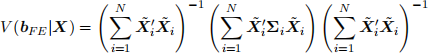
where 
(b) Discuss the relationship between the covariance matrix above and the White covariance matrix for the heteroskedastic cross-sectional data.
(c) Propose an estimator for V (bF E|X)
(d) Provide sufficient conditions and establish the consistency of your estimator.
B. Computational problems:
The goal of this problem is to get more familiar with event study designs. You may want to have a look at Goodman-Bacon (2021).
In this problem, you will simulate your own data. Because of this, you will know the underlying data generating process and what the “true” value of the parameters are and will be able to see how far astray the two way fixed effects model can take.
We consider a setting in which all 50 states in the U.S. implement a policy change (all units are eventually treated), but at different times. States are sorted into “treatment groups” depending on when they enacted the policy g ∈ {1986, 1992, 1998, 2004}.
Steps for data-generation:
(1) Start with 1000 units, each denoted by i.
(2) Randomly assign these units to 1 of 50 states (state = {1, 2, 3, . . . , 50}.
(3) Randomly assign each state into one of 4 treatment groups (year of policy enactment)
g ∈ {1986, 1992, 1998, 2004}. Define a variable Gi for what treatment group unit i belongs to: Gi ∈ {1986, 1992, 1998, 2004}.
(4) For each unit, simulate outcome data from 1980 to 2010 drawn from the following data generating process:
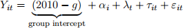
where
• αi are unit fixed effects drawn randomly from 
• λt are time fixed effects generated as

with ε timeFE ∼ N(0, 1).
• εit ∼ N(0,(2/1)2) is an idiosyncratic error term.
• τit are the unit-specific treatment effects at time t generated as
τit = 1 × (t − g + 1) × 1(t ≥ g)
Note that at the time of the event (t = g) the treatment effect is equal to 1 (i.e. the instantaneous treatment effect is 1).
1. Examine the data generating process. Which part of the equation is the ATT? Simulate out the data once (later you will be asked to repeat many times - set a seed!) and graph the ATT for each group in calendar time (i.e. put t on the x-axis).
2. Now plot the ATT in “event time” (i.e. t − g). Are treatment effects homogenous in this setting? Describe the evolution of treatment effects after treatment time.
3. Are you willing to make a parallel trends assumption? What are you willing to assume would have evolved in parallel, compared to what? Why (or why not) do you find this assumption reasonable?
Now we will run TWFE regression using “event study” dummy variables 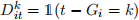 which take value 1 if unit i is k periods away from intitial treatment at time t and 0 otherwise. Your regression should look like this:
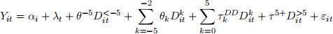
where  Note that we are “leaving out” the dummy for event time k = −1.
Historically (until very recently) people have interpreted τk DD as a measure of the average treatment effect of being exposed to treatment for k periods, and estimates of θk as measures of pre-trends. As we will see, this is not a correct interpretation.
We will perform a Monte Carlo exercise where we generate data according to the data generating process above and estimate the TWFE regression. Repeat this 100 times, saving the values of the thetas and taus each time. (Note that I am asking you to save the thetas and taus, not the corresponding standard erros, so you do not need to worry about how to estimate the standard errors here.)
4. In one graph, plot in “event study” time (1) the Monte Carlo mean for each θk and τk DD, assuming θ−1 = 0 and (2) the true treatment effect over the same event study time (i.e. from -5 to 5). Why are the TWFE regression estimates so off? (Rely on our discussion in class and/or Goodman-Bacon, 2021).
2024-03-04