In this assignment, you will perform color image reconstruction using Bayer pattern and color reproduction using Dithering.

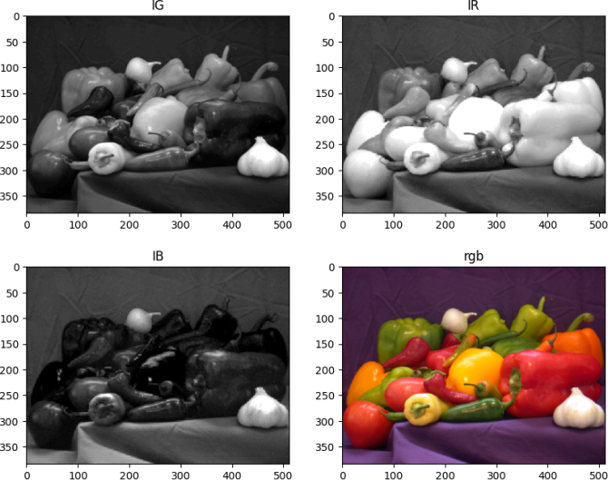
(I) BasicBayer : In this part, you will reconstruct this RGB color image (this original color

image is only for your reference, you will not use it inside your code) given a corresponding Bayer pattern image (your code takes the Bayer pattern as input). The Bayer pattern used is GRBG.

Your task is to reconstruct green, red and blue channels from the Bayer pattern image using these Green, Red, and Blue image masks, where black and white vertices respectively represent valid and empty entries. These masks together form the Bayer color pattern, viz., GRBG.

You should complete the provided template python script to interpolate the empty entries in the reconstructed green, red and blue channels independently of each other. Next, combine  these channels into a full RGB color image and display this image.

Details about Bayer filter and the reconstruction process are provided in the presentation Bayer Filter and Demosaicing.pdf. You can also refer to the Wikipedia pages on Bayer filter and demosaicing.

In case you are interested in even more details, here's a nice reference:

http://www.site.uottawa.ca/~edubois/lslcd/

Note: This assignment requires you to implement a modified version of the interpolation

algorithm, where values from all valid neighbours (shaded pixels in the mask) are averaged.

As a simple scheme of pixel interpolation, you can follow these rules:

●   For reconstruction of the green channel IG with respect to the pattern Green, the values at empty locations can be interpolated as:

○    B = (A+C+F)/3

○    D = (C+H)/2

○ G = (F+C+H+K)/4, etc.

●   For reconstruction of the red channel IR with respect to the pattern Red, use these rules:

○ C = (B+D)/2

○ F = (B+J)/2

○ G = (B+D+L+J)/4, etc.

Note that the fi rst column and the last row are entirely empty. You need to fill them in by copying the second column and the second last row, respectively.

●   For reconstruction of the blue channel IB with respect to the pattern Blue, use these rules:

○    F = (E+G)/2

○ ,I = (E+M)/2

○ J = (E+G+O+M)/4, etc.

Note that here the last column and the fi rst row are entirely empty. You need to fill them by copying the second row and the second last column respectively.

Expected output:

(II) Floyd-Steinberg dithering:

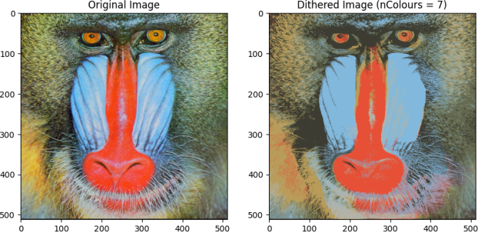
Complete the provided template python script.to read this RGB image and implement Floyd-Steinberg dithering algorithm to change the representation of this image.

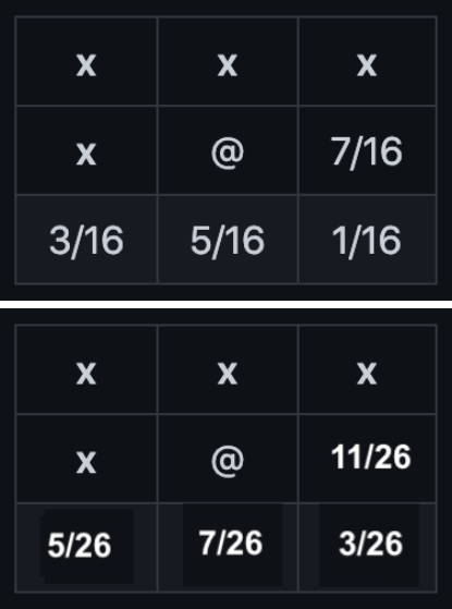
The original algorithm uses the error distribution on the left, but you need to implement the one on the right:

The template script:

●   Dynamically calculates an N-colour palette for the given image (in the notebook the variable nColours determines the number of colours in the palette).

● Uses the KMeans clustering algorithm to determine the best colors.

● Makes a kd-tree palette from the provided list of colors.

● Applies the Floyd-Steinbergmethod to change the representation of the image.

More details about Dithering techniques can be found in the Wikipedia pages onDither and Palette.

Hints:

● Check if x andy are within the image bounds for each pixel location

● Perform the action on each colour channel.

Expected output:

colours:

[[0.91219912 0.3257617  0.21832768]

[0.70676912 0.72203413 0.68072663]

[0.41088001 0.42779406 0.31911404]

[0.52587285 0.73030921 0.87671832]

[0.24926086 0.24574098 0.20012105]

[0.47650788 0.56045069 0.53032372]

[0.7265762 0.62201352 0.36742985]]

Note that you need to adjust the parameters of sklearn.cluster.KMeans till you get the colors given above. Also, the colours found by K-Means depend on the version of scikit-learn so if you are running the code on your own machine, make sure that it has a same python version as cola b (1.2.2). You can install it by running: pip install scikit-learn==1.2.2

(III) Affine Transformation:

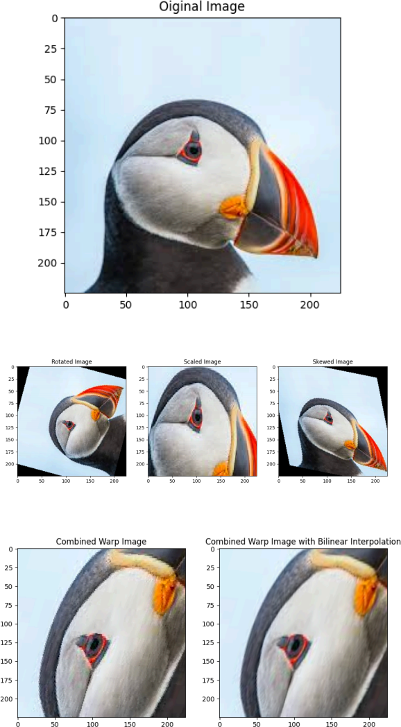
In this part, you will perform image rotation, scaling, and skewing which are specializations of affi ne transformation.

You should complete the provided template python script.

In parts 1 - 4 you are required to create and apply the transformations using your own code. You are not allowed to use built-in functions like skimage.transform.warp for this purpose.

IYou ned to iterate over the pixel locations of the output image ([x_out, y_out]), fi nd the

corresponding location in the input image using the inverse transform ([x_in, y_in] =

inverse-transform(x_out, y_out)), and fill in that pixel value in the output image (output[x_out, y_out] = input[x_in, y_in]).

Note that the obtained [x_in, y_in] are likely floating point values so you can simply take the floor of the obtained values ([int(x_in), int(y_in)]).

In part 5, you will use skimage.transform.warp to obtain the pixel values at the exact     floating point coordinates  [x_in, y_in] using bilinear interpolation over the neighbouring pixels rather than simply taking the pixel value at [int(x_in), int(y_in)].

Read this color image as the input image, and apply the following transformations to the input image independently (not sequentially).

1. ARotation transformation matrix T_r (75 degrees counter-clockwise).

2. AScale transformation matrix T_s which scales the placement of the points by 1.5 times in the x-direction and 2.5 times in the y-direction.

3. A Skew transformation with parameter = 0.2 in both directions.

4. Combination of the transformations in 1, 2, and 3: Affi ne transformation is equivalent to a linear transformation (i.e. multiplying the vectors in homogeneous coordinates by the

augmented matrix). So to combine different affi ne transformations one can multiply the 3x3 matrices of each transformation to arrive at a single 3x3 matrix that corresponds to the combination of the transformations. To demonstrate this, apply the dot product (matrix multiplication) of the previous three transformation matrices to the input image.

5. The above implementation of backwards mapping diminishes the quality of the original image due to the rounding off errors in the floating point coordinates, To address this, apply the combined transformation of part 4 to the input image using skimage.transform.warp through bi linear interpolation. To choose between different interpolation methods, you can pass the argument `order` to skimage.transform.warp.

Expected outputs:

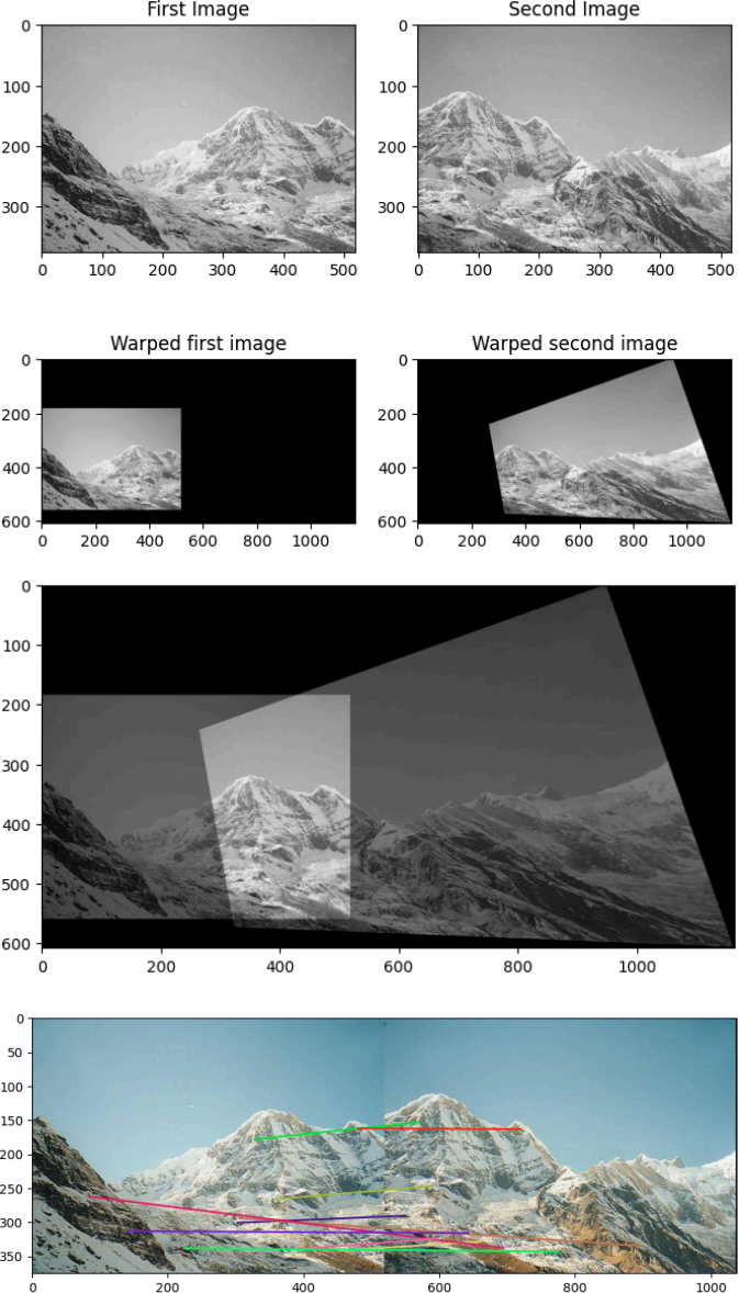
(IV) Image stitching by feature-matching :

In this part, you will perform image stitching by completing this template code. and using    the images im1 and im2 as inputs. The resulting stitched image should look similar to this.

The feature-matching algorithm for image stitching that you need to implement can be briefly summarized as follows:

Step 1) Detect local features with BRIEF or ORB in the two images I1 and I2. You can also use any other feature extractors like SIFT or SURF.

Step 2) Perform feature matching between I1 and I2, based on (approximate) nearest

neighbour search, to generate a set of putative matching feature pairs. Usually, the similarity or distance between two feature descriptors is considered as the metric for matching. For    this step you should use skimage.feature.match_descriptors. This function allows for basic  heuristics to better handle ambiguous matches and potentially discard outliers. In

particular, when calling skimage.feature.match_descriptors you should set the argument

`cross_check` to True and the argument `max_distance` to a proper value that you can fi nd   by hand-tuning. In any case a lot of outliers (i.e. wrong matches) will be selected in this step and step 3 will handle them.

Step 3) A homography matrix is a 3-by-3 matrix that defi nes the transformation between the two images, i.e.,

H12 * [x1, y1, 1]T  = w * [x2, y2, 1]T

where (x1, y1) and (x2, y2) are the image coordinates of the matching features in the two images, H12 is the homography matrix and w is a scalar.

Compute the homography matrix between I1 and I2 based on the matches found in step 2 using the RANSAC algorithm implemented by skimage.measure.ransac. The RANSAC

algorithm is a good choice to fi nd the homography matrix because there are a lot of outlier  matches and RANSAC can handle a lot of outliers. In this step, you may need to hand-tune   the parameters of skimage.measure.ransacso the output of your code becomes consistent and stable.

Step 4) Perform image stitching based on the homography matrix found in step 3. For this, you will need to calculate the new image coordinates for every pixel in I1, with respect to I2  coordinate system. If H12 is calculated correctly, you should expect that after

transformation, the features in I1 now have the same coordinates to their corresponding

features in I2, i.e., they are translated to the matching places.

The resulting stitched image should look similar to this.

Finally, randomly select 10 of the found inlier matches (as returned by the RANSAC

algorithm in step 3), and show them using skimage.feature.plot_matches. The expected output is provide below at the end.

Note that steps 3) and 4) could be correlated. To decide the inliers, we need a model H to  see if the matches fit it. On the other hand, to obtain H, we need sufficient true matches to complete the estimation. This is a chicken-egg problem. Refer to RANSAC if you are interested.

When calculating the new image coordinates, try to avoid using loops to access every pixel since matrix operations are usually much faster than loops.

To make this step easier you time, a reference implementation of stitching with detailed   comments is available in the provided code. You can use it in your code (but may need to modify a bit). You are also welcome to develop your own implementation too.

Note, you need to run your implementation multiple times to make sure the results of ransac are consistent. If they are not, tweak the parameters so that the results become consistent.

Expected output: