Hello, dear friend, you can consult us at any time if you have any questions, add WeChat: daixieit

CI 1871 Excel Exam, Spring 2024

This is an open book and notes exam, but you may NOT discuss the exam with anyone, get help from anyone, or work with anyone. You can use a PC or a Mac.

You must submit to Canvas your ZIPPED exam folder by 6 pm on Mon 26 Feb 2024.

Numbers below in parentheses (#) indicate the point value of each question.

Partial credit is possible so, if a formula does not work, enter your best guess but without the = sign. Formulas must give correct answers if the data change.

1.  On your desktop, create a folder named HWID LastName FirstName Excel Exam S24 (use your own names and HWID). You will store your Excel files in that folder, ZIP it, and submit it to Canvas. So that I can see your formulas, unlike your homework, the files you save to the folder must be Excel files and NOT pdf files.

2.  Download the files I emailed you, aExcelMTOriginalS24 and bExcelMTPivotOriginalS24.

3.  Open aExcelMTOriginalS24. Save it to the HWID LastName FirstName Excel Exam S24 folder using the name cExcel HWID FirstName LastName S24 (use your own data).

Click the Salary worksheet tab.

(4) 4.   In cell A1 type your HWID FirstName LastName.

(4) 5.   Merge and left align cells G1:J1.

(8) 6.   In cell G1, insert a formula that will display and automatically update the current date and

time. Format the cell so that it displays this: It is Hour:Minute AM or PM on Day Date

Month Year. For example, at 6 o’clock in the evening on Monday  26 February 2024 the cell would display It is 6:00 PM on Mon 26 Feb 2024.

(8) 7.  Set a Data Validation for cell C2 so that only whole numbers between 2 and 9, inclusive,  are accepted. Set the Input Message to Enter Rate. Set the error alert to Must be whole number between 2 and 9, inclusive. Set the error alert Style to STOP if an error occurs.

(10) 8.   In cell D6, enter a formula that will display the Department Name based on the Code in C6 and the Codes and Names in C21:D40. So, D6 will show

Finance. If the Code is not in the table, display ***Code Not Found or #N/A

(4) 9.   Fill the formula in cell D6 down to cell D18 and preserve the format.

(6) 10.   In cell F6, enter a formula that will calculate the Commission for Chiu. If his Sales value is  under $15,000, the Commission is the Commission Rate in cell C2 times his Sales in cell E6 divided by 100. Otherwise, it is the Commission Rate in cell C2 times his Sales in cell E6 divided by 100, plus 500 extra.

(4) 11.   Fill the formula in cell F6 down to cell F18 and preserve the format. The Commission for Chiu should be $627 and that for Rodriguez should be $1,275.

(4) 12.   In cell H6, enter a formula that calculates the Total Compensation, which is the Commission plus the Base Salary.

(4) 13.   Fill the formula in cell H6 down to cell H18 and preserve the format.

(4) 14.   In I6:I18 (that is eye 6 not 16), enter a formula that calculates the rank for Total

Compensation for everyone. Display only the rank number. The rank for Chiu is 12.

(8) 15.   In J6:J18, enter a formula that again calculates the rank for Total Compensation for

everyone. Display blue Data Bars without the numbers for the Ranks. Make the borders of the bars orange.

(8) 16.   Set a Conditional Format so that cells with formulas in them will have a red font.

(4) 17.   Split the screen between rows 10 and 11. Scroll the bottom part of the screen so that rows 10 and 15 appear next to each other.

Click the Table worksheet tab.

(4) 18.   In cell E10, enter a formula that finds the sum of E5:E9.

(4) 19.   In cell F5, enter a formula that will calculate the Percent of Grand Total for Veg. That is,

divide the 3 Month Total for Veg by Grand Total in cell E10.

(4) 20.   Fill the formula in F5 down to F9.

(4) 21.   Format cells F5:F9 as a percentage with 0 decimal places.

(4) 22.  Convert the range A4:F10 to a table with the top row designated as headers.

(4) 23.   Name the table Plants.

(4) 24.  Sort the rows 5:9 by Type alphabetically, A to Z.

(8) 25.   Insert a Table Total Row.

(4) 26.   Use the Table Total Row built in formulas to display the Average of the April column.

(4) 27.  Place a heavy purple border around cells A4:F11.

(8) 28.   In cell E11, insert a Column sparkline for cells E5:E9. Make the Sparkline Color orange.

(4) 29.   Place a heavy purple border around the cell with the Sparkline..

(8) 30.   Freeze the pane so that column A and rows 1 through 4 are always on the screen. No other rows or columns should be frozen.

Click the Chart Data worksheet tab. Follow the instructions below to make a chart that looks like this:

The chart has the following characteristics:

(8) 31.  Chart Type: The blue line is a 2-D Line chart with % Fully Vaccinated on the Vertical Axis and State on the Horizontal Axis. Depending on your Excel setup, state names may be vertical or at a slant. Either way is fine.

(4) 32.  Move the chart to its own chartsheet called c1.

(4) 33.  Series Name: Vaccinated

(4) 34.  Chart title: COVID Vaccination Rates and Deaths

(4) 35.  Chart title font is black 14 pt Arial Black.

(4) 36.   Line color is red and 3 pt width.

(4) 37.  Chart and Plot Area: Newsprint texture fill. Choose a different texture if you do not have Newsprint.

Vertical Axis:

(4) 38.  Numbers are red percentages with zero decimal points.

(4) 39.  Scale goes from 0 to 100%

(4) 40.   Numbers are red 9 pt Arial Black.

(4) 41.  Axis Title: Percent Fully Vaccinated.

(4) 42.  Axis Title Font: red 12 pt Arial Black.

(4) 43.  Vertical axis major gridlines: 1 pt black.

(4) 44.  Axis: 3 pt red

Horizontal Axis:

(4) 45.  State names are black 9 pt Arial Black.

(4) 46.  Axis Title: States.

(4) 47.  Axis Title Font: black 12 pt Arial Black.

(4) 48.  Axis: 3 pt black

Secondary Chart (purple line):

(4) 49.  Second Chart Type: The purple line is a 2-D Line chart with Deaths per 100K on the Vertical Axis. This series should be plotted on a Secondary Axis. States should remain on the Horizontal Axis. The series name should be Deaths.

(4) 50.  Secondary line color is purple and 3 pt width.

(4) 51.  Secondary Axis numbers show one decimal point and are purple 9 pt Arial Black.

(4) 52.  Secondary Axis Title: Deaths per 100K.

(4) 53.  Secondary Axis Title Font: purple 12 pt Arial Black.

(4) 54.  Secondary Axis: 3 pt purple

(8) 55.   Insert a text box with the text Lowest Death Rate. Text is purple 12 pt Arial Black.

(8) 56.   Insert a purple arrow with 3 pt weight. Adjust the textbox and arrows as shown above.

Click the Sort worksheet tab.

(8) 57.   In J5:J54, use Flash Fill to display the state names only (without the dash and number).

(8) 58.  Sort the data in rows 5 through 54 by Fully Vaccinated (column H) in ascending order

(smallest to largest) and, within Fully Vaccinated, by State (column A) in descending order (Z to A).

(8) 59.  Change the Mississippi value of Cases, Daily Avg in B5 so Cases Per Vaccinated in I5 (eye five) is exactly 11,000.

(4) 60.   Filter the data so that only rows with Deaths, Daily Ave in col F are between 30 and 50.

Click the Calculations tab.

(8) 61.  Create conditional formats for cells C7:C56 so that:

•  the font will be bold italic red if the Num in Stock is under 30.

•  the fill color will be pink if the Num in Stock is over 50.

(8) 62.  Change the format of the dates in Column D to show the day, date, month, and year. For example, D7 should show Thu 9 Nov 2023.

(4) 63.   Format the numbers in E7:E56 as currency with the dollar sign and 2 decimal places.

(4) 64.   In cell E1, enter a formula that displays the lowest Base Salary on the Salary worksheet.

(8) 65.   In cell E2, enter a formula that displays the number of roses where the Retail Price is over $14.00 and the Num in Stock is under 40.

(8) 66.   In cell E3 enter a formula that displays the sum of the Retail Price where the Num in Stock is over 40 and the Color is Red.

(4) 67.  Create a Named Ranged called Price for the range E7:E56.

(8) 68.   In cell E4, enter a formula that displays the highest Retail Price. Use the named range

Price in your formula. Format the cell so that it displays Highest Price is $xx.xx, where the x’s are the numbers.

(8) 69.   In cell G7, enter a formula that displays Below Ave if the Num in Stock for Sunny Days is

under the average Num in Stock for all roses. Otherwise, display OK.

(10) 70.   In cell H7, enter a formula that displays:

• Order Now if the Num in Stock is 30 or less.

• Order Soon if the Num in Stock is between 30 and 40.

• OK if the Num in Stock is 40 or more.

(4) 71.   Fill the formulas in G7:H7 down to row 56 and preserve the format.

(4) 72.   Hide rows 11:54.

(4) 73.  Arrange the worksheet tabs in this order:

Save the workbook and exit Excel.

Pivot Tables.

74. Open bExcelMTPivotOriginalS24 and save it to the HWID LastName FirstName Excel Exam S24 folder using the name dExcel Pivot HWID FirstName LastName S24, (use your own information).

Click the Data for Table tab.

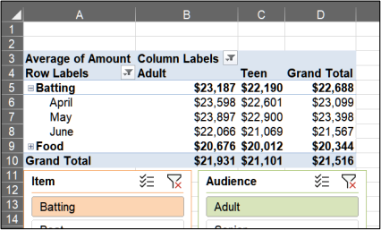
(10) 75.  Construct a PivotTable that has:

• Amount in the Values area

• Item in the Rows area and Month in the Rows area, under Item

• Audience in the Columns area Name the worksheet Amount.

(4) 76.   Insert a Slicer for Item and apply an Orange color design.

(4) 77.   Insert a Slicer for Audience and apply a Green color design.

(8) 78.   Use the slicers to show Item for Batting and Food, and Audience for Adult and Teen.

(4) 79.  Collapse the Food field.

(8) 80.  Display the averages rather than the sum of the Amount. Use the currency style, rounded

to 0 decimal places, and displaying the $.

(2) 81.  Arrange slicers so they are under the table.

Click the Data for Chart worksheet tab.

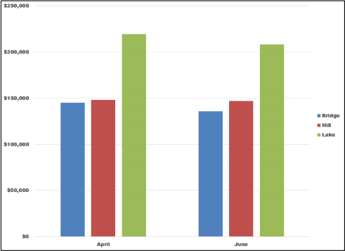
(8) 82.  Construct a PivotTable that has:

• Amount in the Values area

• Month in the Rows area

• Park in the Columns area

Name the worksheet Pivot Table for Chart.

(8) 83.  Create a 2-D Clustered Column chart.

(4) 84.   Move the chart to its own chartsheet. Name the chartsheet Chart1.

(8) 85.   Filter the chart so that it shows the Amount from Bridge, Hill, and Lake for April and June. (4) 86.   Make the font of all the text and numbers on the chart 12 pt Arial Black.

(8) 87.   Make all the numbers currency format, with 0 decimal places.

When done, the chart should look like the following.

(4) 88.  Arrange the worksheet tabs so they are in this order:

Save the workbook and exit Excel.

Submit Your Exam Folder

Your exam folder should have the following two Excel files in it. The files must be Excel files and NOT pdf files (like your homework).

cExcel HWID FirstName LastName S24

dExcel Pivot HWID FirstName LastName S24

ZIP your HWID LastName FirstName Excel Exam S24 folder and submit it to the Excel Exam assignment folder in Canvas by 6 pm on Monday 26 February 2024.