Modelling and Simulation of Saab 340B Aircraft
Hello, dear friend, you can consult us at any time if you have any questions, add WeChat: daixieit
N-ASD-AVMS: Air Vehicle Modelling and Simulation
Modelling and Simulation of Saab 340B Aircraft
1 Aims
The aim of this assignment is to foster a profound comprehension of the rigorous process required to critically analyse and validate an intricate simulation model within an industrial context. In pursuit of this goal, we have chosen the Saab 340B aircraft as our focal point, employing MATLAB/Simulink (Version 2023a) as our primary tool. More specifically, the aims are:
• To develop an accurate and well-structured MATLAB model of the Saab 340B aircraft dynamics using comprehensive modular code and detailed documentation. The model will simulate the full nonlinear aircraft dynamics and enable trimmed flight condition calculation.
• To thoroughly test, verify and validate the Saab 340B model through comparison of simulated dynamics and trim conditions with known aircraft performance data across the flight envelope. Quantitative metrics will be used to evaluate model accuracy.
• To correctly calculate steady, level-trimmed flight conditions for the Saab 340B model across a range of speeds, altitudes and configurations. To then derive linear state-space models using perturbation methods at various trim points.
• To comprehensively analyse the longitudinal and lateral dynamics and characteristics of the Saab 340B using the nonlinear and linear models. Both time-domain dynamic response and frequency-domain stability analysis techniques will be employed to evaluate handling qualities.
2 Introduction to Aircraft Saab 340B
The Saab 340B aircraft shown in Figure 1, operated by Cranfield University's National Flying Laboratory Centre (NFLC), is a twin-turboprop regional airliner that has been modified for research and teaching purposes. The NFLC Saab 340B, registration G-NFLB, serves as a national research facility for universities across the United Kingdom to conduct flight testing and provide hands-on flight experience for students.

Figure 1 Cranfield’s Saab 340B
The Saab 340B has a maximum cruising speed of 306 knots and a range of up to 1,500 nautical miles. It can carry up to 36 passengers in a standard all-economy class configuration. The aircraft is powered by two Allison AE2100D turboprop engines each producing 1,865 shaft horsepower. Key specifications of the Cranfield Saab 340B include:
Length: 19.76 m
Wingspan: 21.44 m
Height: 7.65 m
Maximum takeoff weight: 14,500 lb
Fuel capacity: 1,741 US gal
The aircraft has been equipped with a research instrumentation system to measure various aircraft parameters during flight testing. This includes air data sensors, accelerometers, rate gyros, control surface position sensors, engine data sensors etc. The instrumentation system allows the collection of high-quality flight test data.
3 Data Provision and Assumptions
The provided aerodynamic model builds upon Cranfield's prior Jetstream J31 Aerodynamic Model, employing the methodology outlined in Wolowicz and Yancey [1] to estimate the propeller slipstream's steady influence on the wing, nacelle, and tailplane. In Appendix A, you will find essential data and files, including modelling files and additional flight test data. There are two sets of flight test data: Part 1, a reduced dataset in Excel format tailored for various dynamic modes (phugoid, roll, spiral, and short-period oscillation), ideal for validating the dynamic performance of the developed model, and Part 2, containing four extended flight test datasets (MATLAB data format) with more variables for comprehensive model validation. Additionally, a file with trim values at various flight conditions is included for comparing trim values between the model and flight test data.
4 Major Tasks (Objectives)
1. Create a generic 6DOF (Euler Angle) simulation by integrating the provided sub-model with your developed sub-subsystems and utilizing other blocks available from the MATLAB Aerospace Blockset and/or MATLAB Function blocks. All blocks have been incorporated into Figure 2, except for the navigation equation block, which you are expected to construct on your own. You can also refer to those equations in Appendix B for additional functions.
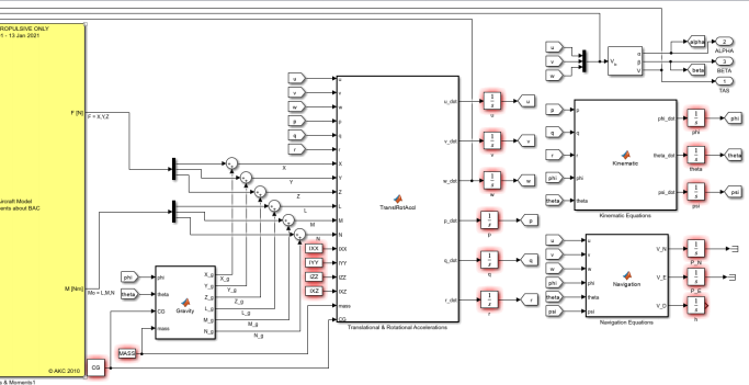
Figure 2 Illustration of blocks including blocks including Gravity, Acceleration, Kinematic, and Navigation blocks
2. Write an initialisation script or function m-file (use Saab340B_initialize_2024A.m.m as a template).
3. Thoroughly test and verify the model by systematically assessing its functionality, ensuring that it runs without any errors, and confirming the accurate implementation of the underlying equations and algorithms. You are expected to define the input and output variables in Simulink for assessment within the MATLAB workspace.
4. Conduct aircraft trim at various chosen flight conditions aligned with the provided trim data file (Flighttest_trimTable_2024A.xlsx. Assess the accuracy of the trim solution by running the model in Simulink for a brief period. Modifications to the model may be necessary to fix specific outputs while allowing for the appropriate states to remain adaptable.
5. Validate the model through a rigorous comparison of trim data and dynamic response data for all aircraft axes with the corresponding data provided in Appendix A, obtained from real-world aircraft. Ensure comprehensive validation of all dynamic modes. Generate dynamic responses by applying identical flight inputs, and carefully consider the impact of the sample rate on determining the simulation's time step.
6. Develop a linear model at a flight condition of your choice, considering the specific parameters and configurations relevant to the selected scenario.
7. Decouple the linear models at various flight conditions (e.g., from low speed to high speed) into longitudinal and lateral/directional models, and visually represent the dynamics modes using an eigenvalue chart. This step helps provide insights into the stability and control characteristics of the aircraft under different conditions.
8. Validate the linear models by conducting detailed comparisons with responses obtained from the full non-linear model, analysing their dynamics modes, or referencing provided flight test data. This validation process ensures that the simplified linear models accurately capture the aircraft's behaviour.
9. Utilize the frequency domain to predict the longitudinal and lateral handling qualities of the aircraft. This analysis allows for a deeper understanding of how the aircraft responds to various inputs and perturbations, helping to assess its overall performance and suitability for specific operational requirements. For example, you need to refer to documents such as ADS-33E-PRF (Figure 6, Page 76) and MIL-HDBK-1797 suggest that the handling qualities of an aircraft can be predicted by analysing its ‘open-loop’ frequency response.
5 Assignment Requirements
The assessment report should consist of the following elements:
1. Begin with a concise yet relevant description of the air vehicle under examination and outline the scope of the assignment, setting the context for the ensuing analysis.
2. Present a data flow diagram illustrating the equations of motion model that you have coded or constructed. Include the equations of motion themselves, alongside either a MATLAB Function block listing or a Simulink diagram. Clearly specify any assumptions made in the development process. Examples from the documentation are the Saab 340B Forces & Moments subsystem and elements exclusively found in the initialization data files. Also, elucidate how you have verified the code's accuracy and reliability.
3. Offer a Simulink diagram that visually represents the simulation model. Supplement this with a comprehensive data dictionary that provides an alphabetical compilation of all additional variables and constants employed within the simulation, excluding those exclusively associated with the Saab 340B Forces & Moments subsystem. Document any additional codes or subsystems you've integrated. List the Simulink library blocks used and provide brief explanations of their purpose and functionality.
4. Delve into the methods employed for trimming the full non-linear model and subsequently present the trim solution. Include examples showcasing the dynamic response of the trimmed model and furnish evidence of its validation, drawing from the provided flight test data. Offer clear, logical explanations for any observed disparities.
5. Present a complete set of transfer functions for the decoupled linear models in their simplest forms. Demonstrate their validation against the full non-linear model, covering both the longitudinal and lateral/directional axes.
6. Present predictions for the frequency response in the pitch and roll channels of the aircraft at your selected flight condition. This section should provide insights into how the aircraft behaves under specific frequency inputs.
7. Include a comprehensive discussion of the results obtained and explore the limitations of the simulation and the exercises undertaken. Reflect on the implications of your findings and consider potential areas for improvement.
Throughout the report, maintain a primary focus on the design, verification, and validation of the model, aiming for high-quality standards. Emphasize a robust analysis of the resultant models and simulation responses. Highlight your adherence to rigorous model development procedures and offer convincing evidence that the simulation effectively represents the supplied mathematical model, substantiating its suitability as a representation of the Saab 340B aircraft.
6 Effort and Mark Scheme
This assignment is expected to require approximately 60 hours of continuous effort for the average student. It is advisable to carefully allocate your time across different aspects of the assignment and adhere to this schedule. Collaboration among students to establish a shared simulation environment is allowed, as long as each individual produces their own written report and acknowledges any collaborative efforts in their respective reports.
The marks given to each task are below.
Task Marks
1. Introduce the assignment and the aircraft 5
2. Construct, verify and document the equations of motion subsystem 15
3. Construct and describe the simulation model 10
4. Trim the nonlinear model and compare the value with flight test data 10
5. Validate the fidelity of the nonlinear model both statically and dynamically using flight test data 20
6. Linearise the model and obtain an appropriate set of transfer functions. Validate the linear model against the non-linear version or flight test data 15
7. Produce a suitable Bode plot and analyse the longitudinal and lateral frequency response 10
8. Summarise the findings on the exercises and present conclusions 5
Report: Style & presentation 10
TOTAL 100
2024-02-26