Nonlinear econometrics for finance HOMEWORK 2
Hello, dear friend, you can consult us at any time if you have any questions, add WeChat: daixieit
Nonlinear econometrics for finance
HOMEWORK 2
(LIE, NLS and GMM)
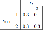
Problem 1 (Law of Iterated Expectations.) (6 points) A financial analyst wants to predict the return on a portfolio. The portfolio gives either a return of 1 or 2 percent in each period. She only knows that the joint probability of returns at time t and t + 1 is
Questions:
1. (2 points) Compute the unconditional expected value E(rt+1).
2. (2 points) Compute the conditional expected value Et(rt+1) = E(rt+1|rt).
3. (2 points) Verify the law of iterated expectations. In particular, show - numerically - that E(rt+1) = E[E(rt+1|rt)].
Note: you can use my document “Examples for the LIE” under Lecture Notes on OneDrive to solve this problem.
Problem 2 (Nonlinear least squares, NLS.) (70 Points) Consider the model:

where qt is output/production, kt is capital and lt is labor. This is the typical specification of a Cobb-Douglas production function.
The parameter θ1 is a proportionality factor capturing “total factor pro-ductivity,” the impact on output/production of factors other than capital and labor. The parameters θ2 and θ3 capture the “output elasticity” of capital and labor, respectively. This is easy to see:
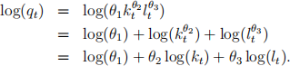
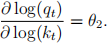
Now, if we take a derivative of, say, the logarithm of output (qt) with respect to the logarithm of capital (kt), we obtain
Because I am multiplying and dividing by the same object, this is, however, the same as:
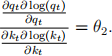
Now, notice that  and
and  are just the derivative of log(qt) with respect to qt (namely,
  ) and the derivative of log(kt) with respect to kt (namely,
  ). Thus,

which means that θ2 measures the “percentage change in output” given a “percentage change in capital”. This is “the elasticity of output with respect to capital”. It addresses the question: if capital increases by 1%, say, what is the percentage increase in output? The answer is: θ21%.
Importantly, we expect θ2 to be smaller than 1. The idea is that a change in capital does not yield a one-to-one change in output. If, for example, θ2 = 0.5, a 1% change in capital would translate into a 0.5% change in output. Naturally, θ3 has the exact same interpretation (for labor) and we are also expecting θ3 to be smaller than 1.
One interesting assumption to test is whether θ2 +θ3 = 1. This is called a case of “constant returns to scale”. What does it mean? Assume we change all inputs by ψ multiplicatively. Then, we are also changing the output by the same amount:

The case θ2 + θ3 > 1 is called “increasing returns to scale” (if we scale all inputs by ψ we are scaling output by more). The case θ2 + θ3 < 1 is called “decreasing returns to scale” (if we scale all inputs by ψ we are scaling output by less).
Questions:
1. (20 Points) Adapt my code for nonlinear least squares with two param-eters to estimate the model with three parameters in Eq. (1) using the Mizon data.
2. (20 Points) Report (1) estimates, (2) standard errors and (3) p values for the three parameters and comment on the statistical significance of your estimates.
3. (10 Points) Comment on the economic significance of your estimates as I did in the discussion above: are θ2 and θ3 positive and smaller than 1? What does it mean?
4. (10 Points) Test for “constant returns to scale” by testing H0 : θ2+θ3 = 1.
5. (10 Points) Test for “constant returns to scale” by testing H0 : θ2 = 0.2 and θ3 = 0.8.
Note: you can use my document “Asymptotic theory and testing” under Lecture Notes on OneDrive to double check the construction of your tests.
Problem 3 (Generalized Method of Moments, GMM.) (24 Points) Use my GMM code to test the following three hypothesis (using optimal second-stage estimates):
1. (10 Points) H0 : θ1 =
θ2.
2. (10 Points) H0 : θ1 = 0.9 and θ2 = 50.
3. (4 Points) Test if the pricing errors are zero.
Note: you can use my document “Asymptotic theory and testing” under Lecture Notes on OneDrive to double check the construction of your tests.
2024-02-26