Hello, dear friend, you can consult us at any time if you have any questions, add WeChat: daixieit

CS 83/183, Winter 2024

Programming Assignment 3

3D Reconstruction

Due Date: (Sunday) February 18, 2023 23:59 (ET)

Instructions

1. Integrity and collaboration: Students are encouraged to work in groups but each student must write their own code and write-up. If you work as a group, include the names of your collaborators in your write up. Code should NOT be shared or copied. Please DO NOT use external code or large-language models such as chatgpt unless permitted. Plagiarism is strongly prohibited and may lead to failure of this course.

2. Start early! Especially if you are not familiar with Python.

3. Questions: If you have any question, please look at piazza first. Other students may have encountered the same problem, and is solved already. If not, post your question on the discussion board. TAs will respond as soon as possible.

4. Write-up: Items to be included in the writeup are mentioned in each question, and summarized in the Writeup section. Please note that we DO NOT accept handwritten scans for your write-up in this assignment. Please type your answers to theory questions and discussions for experiments electronically.

5. Handout: The handout zip file contains 3 items. assgn3.pdf is the assignment handout. data contains 2 temple image files from the Middlebury MVS Temple Data set, and some npz files. python contains the scripts that you will make use of in this homework.

6. Submission: Your submission for this assignment should be a zip file, <dartmouthID>.zip, composed of your write-up, your Python implementations (including helper functions), and your implementations, results for extra credit (optional). Your final upload should have the files arranged in this layout:

• <dartmouthID>.zip

– <dartmouthID>.pdf

– python

∗ submission.py (provided)

∗ helper.py (provided)

∗ project cad.py (provided)

∗ test depth.py (provided)

∗ test params.py (provided)

∗ test pose.py (provided)

∗ test rectify.py (provided)

∗ test temple coords.py (provided)

– data

∗ im1.png (provided)

∗ im2.png (provided)

∗ intrinsics.npz (provided)

∗ some corresp.npz (provided)

∗ temple coords.npz (provided)

∗ pnp.npz (provided)

∗ extrinsics.npz (generate)

∗ rectify.npz (generate)

Please make sure you do follow the submission rules mentioned above before uploading your zip file to Canvas. Assignments that violate this submission rule will be penalized by up to 10% of the total score.

1 Overview

One of the major areas of computer vision is 3D reconstruction. Given several 2D images of an environment, can we recover the 3D structure of the environment, as well as the position of the camera/robot? This has many uses in robotics and autonomous systems, as understanding the 3D structure of the environment is crucial to navigation. You don’t want your robot constantly bumping into walls, or running over human beings!

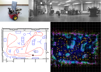
Figure 1: Example of a robot using SLAM, a 3D reconstruction and localization algorithm

In this assignment there are two programming parts: sparse reconstruction and dense re-construction. Sparse reconstructions generally contain a number of points, but still manage to describe the objects in question. Dense reconstructions are detailed and fine grained. In fields like 3D modelling and graphics, extremely accurate dense reconstructions are invalu-able when generating 3D models of real world objects and scenes.

In Part 1, you will be writing a set of functions to generate a sparse point cloud for some test images we have provided to you. The test images are 2 renderings of a temple from two different angles. We have also provided you with a npz file containing good point correspondences between the two images. You will first write a function that computes the fundamental matrix between the two images. Then write a function that uses the epipolar constraint to find more point matches between the two images. Finally, you will write a function that will triangulate the 3D points for each pair of 2D point correspondences.

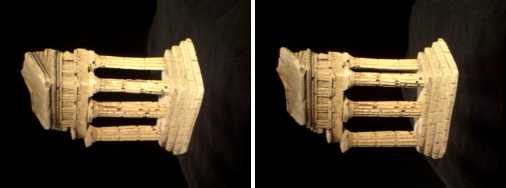
Figure 2: The two temple images we have provided to you

We have provided you with a few helpful npz files. The file data/some corresp.npz contains good point correspondences. You will use this to compute the Fundamental ma-trix. The file data/intrinsics.npz contains intrinsic camera matrices, which you will need to compute the full camera projection matrices. Finally, the file data/temple_coords.npz contains some points on the first image that should be easy to localize in the second image.

In Part 2, we utilize the extrinsic parameters computed by Part 1 to further achieve dense 3D reconstruction of this temple. You will need to compute the rectification parame-ters. We have provided you with test_rectify.py (and some helper functions) that will use your rectification function to warp the stereo pair. You will then optionally use the warped pair to compute a disparity map and finally a dense depth map.

In both cases, multiple images are required, because without two images with a large portion overlapping the problem is mathematically underspecified. It is for this same reason biologists suppose that humans, and other predatory animals such as eagles and dogs, have two front facing eyes. Hunters need to be able to discern depth when chasing their prey. On the other hand herbivores, such as deer and squirrels, have their eyes position on the sides of their head, sacrificing most of their depth perception for a larger field of view. The whole problem of 3D reconstruction is inspired by the fact that humans and many other animals rely on dome degree of depth perception when navigating and interacting with their environment. Giving autonomous systems this information is very useful.

2 Sparse Reconstruction

In this section, you will be writing a set of function to compute the sparse reconstruction from two sample images of a temple. You will first estimate the Fundamental matrix, com-pute point correspondences, then plot the results in 3D.

It may be helpful to read through Section 2.5 right now. In Section 2.5 we ask you to write a testing script that will run your whole pipeline. It will be easier to start that now and add to it as you complete each of the questions one after the other.

2.1 Implement the eight point algorithm (10 points)

In this question, you’re going to use the eight point algorithm which is covered in class to estimate the fundamental matrix. Please use the point correspondences provided in data/some corresp.npz; you can load and view the contents of a .npz file as follows:

data = np . l o a d ( ” . . / data / s om e c o r r e s p . npz ” )

print ( data . f i l e s )

Write a function with the following signature:

F = eight_point(pts1, pts2, M)

where pts1 and pts2 are N × 2 matrices corresponding to the (x,y) coordinates of the N points in the first and second image respectively, and M is a scale parameter.

• Normalize points and un-normalize F: You should scale the data by dividing each co-ordinate by M (the maximum of the image’s width and height) using a transformation matrix T. After computing F, you will have to “unscale” the fundamental matrix. If xnorm = T x, then Funnorm = T TF T. (Note: This formula should not be confused with how homography normalization was done in assignment 2.)

• You must enforce the rank 2 constraint on F before unscaling. Recall that a valid fundamental matrix F will have all epipolar lines intersect at a certain point, meaning that there exists a non-trivial null space for F. In general, with real points, the eight-point solution for F will not come with this condition. To enforce the rank 2 constraint, decompose F with SVD to get the three matrices U, Σ, V such that F = UΣVT . Then force the matrix to be rank 2 by setting the smallest singular value in Σ to zero, giving you a new Σ'. Now compute the proper fundamental matrix with F' = UΣ'VT .

• You may find it helpful to refine the solution by using local minimization. This probably won’t fix a completely broken solution, but may make a good solution better by locally minimizing a geometric cost function. For this we have provided a helper function refineF in helper.py taking in F and the two sets of points, which you can call from eight_point before unscaling F.

• Remember that the x-coordinate of a point in the image is its column entry and y-coordinate is the row entry. Also note that eight-point is just a figurative name, it just means that you need at least 8 points; your algorithm should use an over-determined system (N > 8 points).

• To visualize the correctness of your estimated F, use the function displayEpipolarF in python/helper.py, which takes in F, and the two images. This GUI lets you select a point in one of the images and visualize the corresponding epipolar line in the other image (Figure 3).

In your write-up: Please include your recovered F and the visualization of some epipo-lar lines (similar to Figure 3).

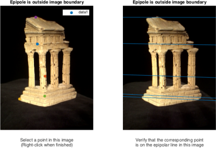
Figure 3: Epipolar lines visualization from displayEpipolarF

2.2 Find epipolar correspondences (20 points)

To reconstruct a 3D scene with a pair of stereo images, we need to find many point pairs. A point pair is two points in each image that correspond to the same 3D scene point. With enough of these pairs, when we plot the resulting 3D points, we will have a rough outline of the 3D object. You found point pairs in the previous homework using feature detectors and feature descriptors, and testing a point in one image with every single point in the other image. But here we can use the fundamental matrix to greatly simplify this search.

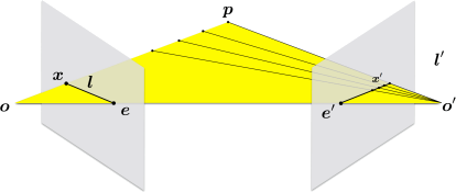
Figure 4: Epipolar Geometry (source Wikipedia)

Recall from class that given a point x in one image (the left view in Figure 4). Its corresponding 3D scene point p could lie anywhere along the line from the camera center o to the point x. This line, along with a second image’s camera center o 0 (the right view in Figure 4) forms a plane. This plane intersects with the image plane of the second camera, resulting in a line l 0 in the second image which describes all the possible locations that x may be found in the second image. Line l 0 is the epipolar line, and we only need to search along this line to find a match for point x found in the first image. Write a function with the following signature:

pts2 = epipolar_correspondences(im1, im2, F, pts1)

where im1 and im2 are the two images in the stereo pair, F is the fundamental matrix computed for the two images using your eight point function, pts1 is a N × 2 matrix containing the (x, y) points in the first image, and the function should return pts2, a N × 2 matrix, which contains the corresponding points in the second image.

• To match one point x in image 1, use fundamental matrix to estimate the corresponding epipolar line l' and generate a set of candidate points in the second image.

• For each candidate points x', a similarity score between x and x' is computed. The point among candidates with highest score is treated as epipolar correspondence.

• There are many ways to define the similarity between two points. Feel free to use whatever you want and describe it in your write-up. One possible solution is to select a small window of size w around the point x. Then compare this target window to the window of the candidate point in the second image. For the images we gave you, simple Euclidean distance or Manhattan distance should suffice.

• Remember to take care of data type and index range.

You can use the function epipolarMatchGUI in python/helper.py to visually test your function. Your function does not need to be perfect, but it should get most easy points correct, like corners, dots etc.

In your write-up: Please include a screenshot of epipolarMatchGUI running with your implementation of epipolar_correspondences (similar to Figure 5). Mention the similarity metric you decided to use. Also comment on any cases where your matching algorithm consistently fails, and why you might think this is.

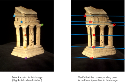
Figure 5: Epipolar Match visualization. A few errors are alright, but it should get most easy points correct (corners, dots, etc.)

2.3 Write a function to compute the essential matrix (10 points)

In order to get the full camera projection matrices we need to compute the Essential matrix. So far, we have only been using the Fundamental matrix. Write a function with the following signature:

E = essential_matrix(F, K1, K2)

Where F is the Fundamental matrix computed between two images, K1 and K2 are the intrinsic camera matrices for the first and second image respectively (contained in data/intrinsics.npz), and E is the computed essential matrix. The intrinsic camera pa-rameters are typically acquired through camera calibration. Refer to the class slides for the relationship between the Fundamental matrix and the Essential matrix.

In your write-up: Please include your estimated E matrix for the temple image pair.

2.4 Implement triangulation (20 points)

Write a function to triangulate pairs of 2D points in the images to a set of 3D points with the signature:

pts3d = triangulate(P1, pts1, P2, pts2)

Where pts1 and pts2 are the N × 2 matrices with the 2D image coordinates, P1 and P2 are the 3×4 camera projection matrices and pts3d is an N ×3 matrix with the correspond-ing 3D points (in all cases, one point per row). Remember that you will need to multiply the given intrinsic matrices with your solution for the extrinsic camera matrices to obtain the final camera projection matrices. For P1 you can assume no rotation or translation, so the extrinsic matrix is just [ I | 0 ]. For P2, pass the essential matrix to the provided function camera2 in python/helper.py to get four possible extrinsic matrices. You will need to de-termine which of these is the correct one to use (see hint in Section 2.5). Refer to the class slides for one possible triangulation algorithm. Once implemented, check the performance by looking at the re-projection error. To compute the re-projection error, project the estimated 3D points back to the image 1 and compute the mean Euclidean error between projected 2D points and the given pts1.

In your write-up: Describe how you determined which extrinsic matrix is correct. Note that simply rewording the hint is not enough. Report your re-projection error using the given pts1 and pts2 in data/some corresp.npz. If implemented correctly, the re-projection error should be less than 2 pixels.

2.5 Write a test script that uses data/temple_coords.npz   (10 points)

You now have all the pieces you need to generate a full 3D reconstruction. Write a test script python/test temple coords.py that does the following:

1. Load the two images and the point correspondences from data/some corresp.npz

2. Run eight point to compute the fundamental matrix F

3. Load the points in image 1 contained in data/temple_coords.npz and run your epipolar_correspondences on them to get the corresponding points in image 2

4. Load data/intrinsics.npz and compute the essential matrix E.

5. Compute the first camera projection matrix P1 and use camera2 to compute the four candidates for P2

6. Run your triangulate function using the four sets of camera matrix candidates, the points from data/temple_coords.npz and their computed correspondences.

7. Figure out the correct P2 and the corresponding 3D points. Hint: You’ll get 4 projection matrix candidates for camera2 from the essential matrix. The correct configuration is the one for which most of the 3D points are in front of both cameras (positive depth).

8. Use matplotlib’s scatter function to plot these point correspondences on screen.

9. Save your computed extrinsic parameters (R1,R2,t1,t2) to data/extrinsics.npz. These extrinsic parameters will be used in the next section.

We will use your test script to run your code, so be sure it runs smoothly. In particular, use relative paths to load files, not absolute paths.

In your write-up: Include 3 images of your final reconstruction of the points given in the file data/temple_coords.npz, from different angles as shown in Figure 6.

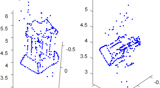
Figure 6: Sample Reconstructions

3 Dense Reconstruction

In applications such as 3D modelling, 3D printing, and AR/VR, a sparse model is not enough. When users are viewing the reconstruction, it is much more pleasing to deal with a dense reconstruction. To do this, it is helpful to rectify the images to make matching easier.

In this section, you will be writing a set of functions to perform a dense reconstruction on our temple examples. Given the provided intrinsic and computed extrinsic parameters, you will need to write a function to compute the rectification parameters of the two images. The rectified images are such that the epipolar lines are horizontal, so searching for corre-spondences becomes a simple linear. This will be done for every point. Finally, you can compute the disparity and depth map.

3.1 Image Rectification (10 points)

Write a program that computes rectification matrices.

M1,M2,K1p,K2p,R1p,R2p,t1p,t2p = rectify pair(K1,K2,R1,R2,t1,t2)

This function takes the left (K1,R1,t1) and right camera parameters (K2,R2,t2), and returns the left (M1) and right (M2) rectification matrices and the updated camera param-eters (K1p,R1p,t1p,K2p,R2p,t2p). You can test your function using the provided script python/test rectify.py. From what we learned in class, the rectify pair function should consecutively run the following steps:

1. Compute the optical centers c1 and c2 of each camera by ci = −(KiRi)−1(Kiti)

2. Compute the new rotation matrix  = [r1 r2 r3]T where r1, r2, r3 ∈ R3×1 are or-thonormal vectors that represent x, y, and z axes of the camera reference frame, respectively.

(a) The new x-axis (r1) is parallel to the baseline: r1 = (c1 − c2)/||c1 − c2||

(b) The new y-axis (r2) is orthogonal to x and to any arbitrary unit vector, which we set to be the z unit vector of the old left matrix: r2 is the cross product of R1(3, :)T and r1

(c) The new z-axis (r3) is orthogonal to x and y: r3 is the cross product of r2 and r1

Set the new rotation matrices as R'1 = R'2 = 

3. Compute the new intrinsic parameters as K01 = K02 = K2

4. Compute the new translation vectors as t1 = −c1 and t2 = −c2

5. Finally, the rectification matrices of the cameras (M1,M2) can be obtained by

Mi = (K'iR'i)(KiRi)−1

Once you finished, run python/test_rectify.py (Ensure data/extrinsics.npz is saved by your python/test_temple_coords.py). This script will test your rectification code on the temple images using the provided intrinsic parameters and your computed extrinsic param-eters. It will also save the estimated rectification matrices and updated camera parameters in data/rectify.npz, which will be used by the function python/test_depth.py.

In your write-up: Include a screenshot of the result of python/test_rectify.py on the temple images. The results should show some epipolar lines that are perfectly horizontal, with corresponding points in both images lying on the same line.

3.2 Dense window matching to find per pixel disparity (20 points)

Write a program that creates a disparity map from a pair of rectified images.

dispM = get_disparity(im1,im2,max disp,win_size)

where max_disp is the maximum disparity and win size is the window size. The output dispM has the same dimension as im1 and im2. Since im1 and im2 are rectified, computing correspondences is reduced to a 1D search problem. The value of dispM(y, x) is given by

where,

and w = (win size−1)/2. This summation on the window can be easily computed by using the scipy.signal.convolve2d function (i.e. convolution with a mask of ones). Note that this is not the only way to implement this.

3.3 Depth map (10 points)

Write a function that creates a depth map from a disparity map.

depthM = get_depth(dispM,K1,K2,R1,R2,t1,t2)

where we can use the fact that

where b is the baseline and f is the focal length of camera. For simplicity, assume that b = ||c1−c2|| (i.e., distance between optical centers) and f = K1(1, 1). Finally, let depthM(y, x) = 0 whenever dispM(y, x) = 0 to avoid division by 0. You can now test your disparity and depth map functions using python/test_depth.py. Ensure that the rectification is saved (by running python/test_rectify.py). This function will rectify the images, then compute the disparity map and the depth map.

In your write-up: Please include images of the disparity and depth maps.

4 Pose Estimation

In this section, you will implement what you have learned in class to estimate the intrinsic and extrinsic parameters of camera given 2D points x on image and their corresponding 3D points X. In other words, given a set of matched points {Xi , xi} and camera model

we want to find the estimate of the camera matrix P ∈ R3×4 , as well as intrinsic parameter matrix K ∈ R3×3 , camera rotation R ∈ R3×3 and camera translation t ∈ R3 , such that

P = K [R t]                                (5)

4.1 Estimate camera matrix P (10 points)

CS 83—Extra credit (optional)

CS183—Part of the assignment (mandatory)

Write a function that estimates the camera matrix P given 2D and 3D points x, X.

where x is 2 × N matrix denoting the (x, y) coordinates of the N points on the image plane and X is 3×N matrix denoting the (x, y, z) coordinates of the corresponding points in the 3D world. Recall that this camera matrix can be computed using the same strategy as homography estimation by Direct Linear Transform (DLT). Once you finish this function, you can run the provided script python/test_pose.py to test your implementation.

In your write-up: Please include the output of the script python/test_pose.py.

4.2 Estimate intrinsic/extrinsic parameters (20 points)

CS 83—Extra credit (optional)

CS183—Part of the assignment (mandatory)

Write a function that estimates both intrinsic and extrinsic parameters from camera matrix.

K, R, t = estimate_params(P)

From what we learned on class, the estimate_params function should consecutively run the following steps:

1. Compute the camera center c by using SVD. Hint: c is the eigenvector corresponding to the smallest eigenvalue.

2. Compute the intrinsic K and rotation R by using QR decomposition. K is a right upper triangle matrix while R is a orthonormal matrix.

3. Compute the translation by t = −Rc.

Once you finish your implementation, you can run the provided script python/test_params.py.

In your write-up: Please include the output of the script python/test_params.py.

4.3 Project a CAD model to the image (20 points)

CS 83—Extra credit (optional)

CS183—Extra credit (optional)

Now you will utilize what you have implemented to estimate the camera matrix from a real image, shown in Figure 7 (left), and project the 3D object (CAD model), shown in Figure 7 (right), back on to the image plane. Write a script python/project_cad.py that does the following:

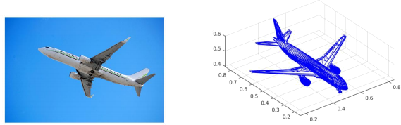
Figure 7: The provided image and 3D CAD model

1. Load an image image, a CAD model cad, 2D points x and 3D points X from the data file data/pnp.npz.

2. Run estimate pose and estimate_params to estimate camera matrix P, intrinsic ma-trix K, rotation matrix R, and translation t.

3. Use your estimated camera matrix P to project the given 3D points X onto the image.

4. Plot the given 2D points x and the projected 3D points on screen. An example is shown in Figure 8 (left).

5. Draw the CAD model rotated by your estimated rotation R on screen. An example is shown in Figure 8 (middle).

6. Project the CAD’s all vertices onto the image and draw the projected CAD model overlapping with the 2D image. An example is shown in Figure 8 (right).

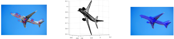
Figure 8: Project a CAD model back onto the image. Left: the image annotated with given 2D points (blue circle) and projected 3D points (red points); Middle: the CAD model rotated by estimated R; Right: the image overlapping with projected CAD model.

In your write-up: Please include the three images similar to Figure 8. You must use different colors from Figure 8. For example, green circle for given 2D points, black points for projected 3D points, blue CAD model, and red projected CAD model overlapping on the image. You will get NO credit if you use the same color.