Hello, dear friend, you can consult us at any time if you have any questions, add WeChat: daixieit

Take-Home Quiz Three

ECE 271B - Winter 2024

Department of Electrical and Computer Engineering

In this quiz, we study the boosting algorithm. This is an iterative procedure that, given a training set {(xi , yi)} ni=1, where yi ∈ {−1, 1}, and a definition of empirical risk

implements the following steps at iteration t:

❼ dataset reweighting: each training example xi receives a non-negative weight ωi ;

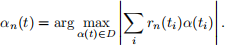
❼ weak learner selection: a weak learner αt(x) is selected from a set of functions U, so as to optimize a function that depends on all examples xi and their weights ωi ;

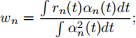
❼ step-size: a step-size wt is computed according to

❼ update: the ensemble learner is updated to

gt+1(x) = gt(x) + wtαt(x).                                                      (3)

Problem 1. (15 points) In this problem, we consider a monotonically decreasing loss function φ(·).

a) (3 points) Derive the equations for the reweighting and weak learner selection steps of the boosting algorithm. Note that, to receive full credit, you must derive the most detailed equation possible. For example, what is an expression for the weights?

b) (3 points) In class, we introduced the Perceptron loss

φ(v) = max(−v, 0).

What is the expression of the boosting weights ωi for this loss?

c) (3 points) Assume that the Perceptron loss is used and the set U is the set of functions

u(x) = wT x,

parametrized by a unit vector w (i.e. ||w|| = 1) with the dimension of x. Derive the boosting algorithm for this scenario.

d) (3 points) Compare the algorithm of c) to the Perceptron learning algorithm. Give a detailed discussion of the similarities and differences.

e) (3 points) Consider the generic boosting algorithm of a). Could this algorithm work with the 0/1-loss?

Problem 2. (12 points) We have seen that neural networks are frequently trained with the entropy loss

L(x, z) = −z log σ[g(x)] − (1 − z) log(1 − σ[g(x)]),

where z ∈ {0, 1} is the class label of example x and

is the sigmoid non-linearity.

a) (4 points) Note that labels z ∈ {0, 1} can be converted to labels y ∈ {−1, 1} with the simple transformation y = 2z − 1. Show that, when this relationship holds, the entropy loss can be written as

L(x, y) = log(1 + e−yg(x)).              (4)

Using this equivalence, what can you say about the ability of neural networks to enforce margins? Are they likely to produce classifiers of large margin? Why?

b) (4 points) Derive the boosting algorithm of 1a) for the loss function of (4). Note that, to receive full credit, you must derive the most detailed equation possible.

c) (4 points) In class, we have derived a similar algorithm for the exponential loss, i.e. for φ(v) = e−v . Compare the two algorithms and discuss how they differ. For which type of problems would it make a difference to use one algorithm vs. the other? Why?

Problem 3. (15 points) In this problem, we consider the AdaBoost algorithm with classification weak learners, i.e. αt(x) ∈ {−1, 1}.

a) (5 points) Consider the implementation of the algorithm using decision stumps as weak learners, i.e.

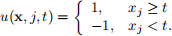
Let U be the set of all weak learners such that t belongs to a pre-defined set of T thresholds. Assume that, for each weak learner, there is also a weak learner of opposite polarity, i.e. u 0 (x, j, t) = −u(x, j, t). For x ∈ Rd , what is the complexity of the boosting algorithm?

b) (5 points) Rather than decision stumps, it was decided to implement weak learners as

u(x;t) = sgn[wT x − t],

where w is computed by linear discriminant analysis. Derive all equations needed to implement the weak learner selection step.

c) (5 points) Repeat b) for weak learners implemented with a Gaussian classifier, i.e. that implement the BDR under the assumption of two Gaussian classes of mean µi , covariance Σi , and probability πi , i ∈ {−1, 1}. The parameters of the Gaussians are learned by maximum likelihood.

Problem 4. (15 points) A classical problem of signal processing is the problem of decomposing a signal f(t) into a combination of functions αn(t) so that

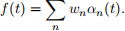
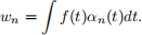
When the functions αn(t) form an orthonormal basis of the space of functions f(t), this is fairly straightforward. It suffices to compute the projections

For example, this is the case of the Fourier series expansion, where the basis functions αn(t) are cosines of multiple frequencies. The problem is, however, more complex when the functions αk(t) form an overcomplete dictionary D, i.e. they are not linearly independent.

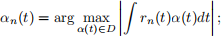
A commonly used algorithm to solve this problem is the matching pursuit algorithm. A residual function r(t) is first initialized with r0(t) = f(t). The algorithm then iterates between the following steps:

❼ find

❼ compute

❼ update the residual

rn+1(t) = rn(t) − wnαn(t).

For a discrete-time signal, sampled at times ti , the dot-products become summations, e.g.

Show that the matching pursuit algorithm is really just an implementation of boosting on a training set {(ti , f(ti))} with weak learners αk(t) and loss function L(y, g(x)) = (y − g(x))2 .

Problem 5. (43 points) In this problem, we will use boosting to, once again, classify digits. In all questions, you will use the training set contained in the directory MNISTtrain (60, 000 examples) and the test set in the directory MNISTtest (10, 000). To reduce training time, we will only use 20, 000 training examples. To read the data, you should use the script readMNIST.m (use readDigits=20, 000 or readDigits=10, 000 respectively, and offset=0). This returns two matrices. The first (imgs) is a matrix with n ∈ {10000, 20000} rows, where each row is a 28 × 28 image of a digit, vectorized into a 784-dimensional row vector. The second (labels) is a matrix with n ∈ {10000, 20000} rows, where each row contains the class label for the corresponding image in imgs. Since there are 10 digit classes, we will learn 10 binary classifiers. Each classifier classifies one class against all others. For example, classifier 1 assigns label Y = 1 to the images of class 1 and label Y = −1 to images of all other classes. Boosting is then used to learn an ensemble rule

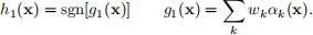
After we learn the 10 rules gi(x), i ∈ {1, . . . , 10}, we assign the image to the class of largest score

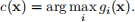
This implementation is called the “one-vs-all” architecture. We will use decision stumps

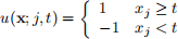
as weak learners. For each weak learner, also consider the “twin” weak learner of opposite polarity

u'(x; j, t) = −u(x; j, t).

This simply chooses the “opposite label” from that selected by u(x; j, t). Note that j ∈ {1, . . . , 784}.

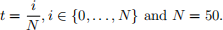
For thresholds, use

a) (10 points) Run AdaBoost for K = 250 iterations. For each binary classifier, plot train and test errors vs. iteration. Report the test error of the final classifier. For each iteration k, store the index of the example of largest weight, i.e. i ∗ = arg maxi wi (k) . At iterations {5, 10, 50, 100, 250} store the margin γi = γ(xi) of each example.

b) (11 points) For each binary classifier, make a plot of cumulative distribution function (cdf) of the margins γi of all training examples after {5, 10, 50, 100, 250} iterations (the cdf is the function F(a) = P(γ ≤ a), and you can do this by computing an histogram and then a cumulative sum of histogram bins.) Comment on what these plots tell you about what boosting is doing to the margins.

c) (11 points) We now visualize the weighting mechanism. For each of the 10 binary classifiers, do the following.

❼ Make a plot of the index of the example of largest weight for each boosting iteration.

❼ Plot the three “heaviest” examples. These are the 3 examples that were most frequently selected, across boosting iterations, as the example of largest weight.

Comment on what these examples tell you about the weighting mechanism.

d) (11 points) We now visualize what the weak learners do. Consider the weak learners αk, k ∈ {1, . . . , K}, chosen by each iteration of AdaBoost. Let i(k) be the index of the feature xi(k) selected at time k. Note that i(k) corresponds to an image (pixel) location. Create a 28 × 28 array a filled with the value 128. Then, for αk, k ∈ {1, . . . , K}, do the following.

❼ If the weak learner selected at iteration k is a regular weak learner (outputs 1 for xi(k) greater than its threshold), store the value 255 on location i(k) of array a.

❼ If the weak learner selected at iteration k is a twin weak learner (outputs −1 for xi(k) greater than its threshold), store the value 0 on location i(k) of array a.

Create the array a for each of the 10 binary classifiers and make a plot of the 10 arrays. Comment on what the classifiers are doing to reach their classification decision.