STAT GR5241 Statistical Machine Learning: Homework 1
Hello, dear friend, you can consult us at any time if you have any questions, add WeChat: daixieit
STAT GR5241 Statistical Machine Learning: Homework 1
Please complete the exercises below.
This homework is due Wednesday, Feb 21, at 8:00 am. Please upload your solution as a pdf file on Courseworks.
Late assignments: For assignments that are submitted within 24 hours of deadline, your grade on the assignment will be calculated by your actual grade on the assignment ×70%. No assignments will be accepted after 24 hours past the original deadline unless under extenuating circumstances.
Problem 1: Risk (30 points)
The following questions all consider a binary classifier f : Rd → {−1, 1}.
(a) To calculate the risk R(f), what function(s) do you need to know, and why? An acceptable answer can write down the form of risk R(f) and describe the components.
(b) Do most machine learning algorithms use risk R(f) or empirical risk R(ˆ)n (f)? Please explain.
(c) If the training data {(˜(x)1 , ˜(y)1 ), ··· , (˜(x)n , ˜(y)n )} for a fixed classifier f are n i.i.d. draws from the true underlying distribution of the data, what is
nl![]() R(f) − R(ˆ)n (f)'?
R(f) − R(ˆ)n (f)'?
Please make a simple argument; no proof is required.
Note: You may assume that R(f) is well behaved such that questions of convergence are all appropriately satisfied. You may also use results from elementary probability.
(d) Under the usual 0 − 1 loss, what is the range of R(f)? With this answer, interpret R(f) in words as a probability (one sentence will suffice).
(e) Training procedure 1 chooses linear classifier f1 entirely at random. Now the risk R(f1 ) is a random variable (a function of the random linear classifier f1 ). What is E[R(f1 )] under the 0 − 1 loss?
(f) Training procedure 2 uses the Perceptron to choose a linear classifier f2 according to a training set {(˜(x)1 , ˜(y)1 ), ··· , (˜(x)n , ˜(y)n )} drawn i.i.d. from the true underlying distribution. By analogy to the previous part, you can consider that training procedure 2 chooses linear classifiers f2 better than entirely at random. Do you expect E[R(f2 )] to be larger or smaller than E[R(f1 )], again under the same 0 − 1 loss?
Problem 2: Bayes Classifier (35 points)
Consider the binary classification problem with the training data set {(x(˜)1 , ˜(y)1 ), (x(˜)2 , ˜(y)2 ), ··· , (x(˜)n , ˜(y)n )}. For
each observation, the class label ˜(y)i ∈ {+1, −1}, and the feature x(˜)i ∈ R2 . We write x(˜)i = (˜(x)![]() , ˜(x)
, ˜(x)![]() ).
).
(a) Assume that we know the class-conditional distributions of the data: p(x|y = +1) is Gaussian with mean vector µ+ and covariance matrix Σ+ and p(x|y = −1) is Gaussian with mean vector µ− and covariance matrix Σ − . Write down the maximum likelihood estimators of µ+ ,µ − , Σ+ , Σ − .
(b) Assume the class-conditional distributions in (a). To find the Bayes-optimal classifier, what function is needed, and how would you estimate this function from the training data? Give the expression of the Bayes-optimal classifier based on this function.
(c) Assume the class-conditional distributions in (a) with Σ+ = Σ − = I2 , where I2 = l0(1) 1(0)] is the identity
matrix (we know Σ+ = Σ − = I2 but don’t know µ+ ,µ − ). Consider the following training data set:
|
i |
˜(y)i |
|
|
|
1 |
+1 |
−1 |
0.7 |
|
2 |
+1 |
1 |
−1.9 |
|
3 |
−1 |
−0.7 |
0.6 |
|
4 |
−1 |
−0.2 |
−1.5 |
A plot of this training data set is shown in the following figure. Train the naive Bayes classifier on this
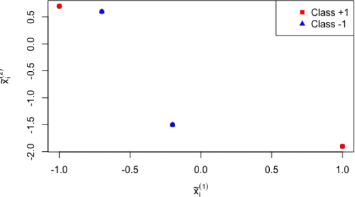
data (please estimate all necessary parameters).
(d) Compute the empirical risk of the classifier in (c) under the 0 − 1 loss.
Problem 3: Perceptron (35 points)
Consider a training data set that consists of three observations (x(˜)1 , ˜(y)1 ), (x(˜)2 , ˜(y)2 ), (x(˜)3 , ˜(y)3 ), where
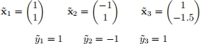
(a) Is the training data linearly separable? Why?
(b) Consider a linear classifier given by an affine hyperplane with normal vector vH =(1(0)) and offset c = 0.
Compute the empirical risk of this classifier (with 0 − 1 loss).
Hint: Check Lecture 3, Page 11 for the linear classifier that corresponds to vH and c. Here, “offset c” means the corresponding linear classifier is given by
fH (x) = sgn(⟨x, vH ⟩ − c).
(c) Suppose that we run the (batch) Perceptron Algorithm as described in Lecture 3, Page 22 (with learning rate α(k) = 1 and gradient computation on Page 23). What is the normal vector vH(′) and the offset c′ of the resulting affine hyperplane after one iteration? Please also compute the empirical risk of the linear classifier that corresponds to this affine hyperplane.
Hint: You may refer to the annotated slides for Lecture 3 for the update rules.
(d) Which cost function does the perceptron cost function approximate, and why do we approximate it?
2024-02-21