ENGN 2820 Spring 2024 Examples 3
Hello, dear friend, you can consult us at any time if you have any questions, add WeChat: daixieit
ENGN 2820 Spring 2024
Examples 3
The due date for this assignment is 11.00 pm Sunday, February 18.
Please submit your assignment as a PDF via the Gradescope link on Canvas. You may submit handwritten answers but please ensure that you work is legible and start the answer to each question on a new page. You may also submit your work using Latex and the source tex file for this assignment is posted on Canvas in ‘Files’.
All the questions refer to an incompressible flow, where ∇ · u = 0, in a fluid of constant density. The standard 2D boundary layer approximation for the region near a wall at y = 0 gives the equations:

1. The flow in a viscous boundary layer over a flat plate at high Reynolds numbers is given by a streamfunction ψ(x, y), where u = ∂ψ/∂y and v = −∂ψ/∂x, that has the form ψ = U0δ(x)f(η). The free-stream velocity outside the layer is (U0, 0), with constant U0. The scale for the boundary layer thickness is δ(x) = (xν/U0) 1/2 and the self-similarity variable is η = y/δ. As shown in the textbook (see Kundu, 4th ed, Sec.10.5), the function f(η) satisfies the nonlinear Blasius differential equation
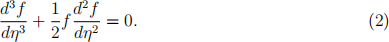
The boundary conditions are that at the wall, y = 0, u = v = 0 corresponding to f = f(1) = 0. At the outer edge of the boundary layer, y/δ → ∞, the streamwise flow matches the free-stream and f (1) = 1. In order to evaluate f(η) and its derivatives we need to obtain a numerical solution to the differential equation.
Look in the folder for Matlab codes on Canvas. There is a sub-folder titled ‘BL-codes’ that contains a Matlab function ‘Blasius BVP.m’, which uses bvp4c to solve this boundary value problem. Read the accompanying notes about bvp4c and its application here.
Use this script to solve for the velocity profile and the other data generated. What are the definitions of the displacement thickness δ ∗ and momentum thickness θ, and give physical interpretations for these? Which one is larger? What is the value of the wall normal velocity v at the outer edge of the boundary layer? Should we consider modifying the original estimate of simple uniform flow (U0, 0) for the outer flow?
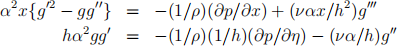
2. Locally, the 2D inviscid flow near a stagnation point is given by the streamfunction ψ = αxy, where α > 0. This satisfies the no-normal flow condition at y = 0, with a slip velocity U0(x) = αx at the wall. We could use a boundary layer approximation to find the viscous near-wall flow, but in fact the flow can be found without this. The flow is given by ψ = αxhg(η), where η = y/h and h is a constant length scale.
• Show that the Navier-Stokes equations give the u, v-momentum equations,
• What are the three boundary conditions we should specify for g(η)?
• From these equations, why can we conclude that ∂p/∂x is independent of η? By considering the conditions at η >> 1, determine ∂p/∂x.
• Determine the appropriate value of h.
• Verify that the u-momentum equation becomes g ′′′ + gg′′ − g ′2 + 1 = 0.
• What can we say about the relative magnitude of ∂p/∂y compared to ∂p/∂x?
How does this relate to the Reynolds number Re = αx2/ν?
• Modify the Matlab script for the Blasius BL to solve this new problem.
3. Refer to the class notes posted for 02-02-24, when we covered the inviscid dynamics of a vortex tube, aligned with the z-axis, that is stretched in an axisymmetric straining flow (ur, 0, uz) = (−αr, 0, 2αz). Assume that this is a Rankine vortex where the swirl flow is uθ = Ωr, 0 ≤ r ≤ R and R is the radius of the tube. We consider an initial material volume of fluid 0 ≤ z ≤ L0 in the tube with initial radius R = R0. Establish that the angular momentum of this material volume is constant. Show though that the kinetic energy of the fluid grows with the stretching.
4. The theory behind Perturbation Methods based on asymptotic approximations is be-yond the scope of this course. Standard references are the books by Milton van Dyke, A.H. Nayfeh, Kervorkian & Cole, and by E.J. Hinch. Most of these are available from the library. Boundary Layer theory is based on matched asymptotic expansions, whereby two separate asymptotic approximations are found for different parts of the flow and then patched together in an overlap region. (Such patching is also needed in numerical simulations that use different solution methods in different regions.) The following question is based on Hinch (Ch5, Ex 5.1) which illustrates the issues.
The function y(x;ϵ) satisfies
ϵy′′ + (1 + ϵ)y′ + y = 0, 0 ≤ x ≤ 1
The boundary conditions are y(0) = 0, y(1) = e−1 . Find the exact solution to this linear second order differential equation. You may assume that ϵ is small(-ish). Give a sketch of the exact solution. Note that if ϵ = 0, this reduces to a first order differential equation and we can only use one boundary condition.
Find the first term of the outer approximation, applying only the boundary condition at x = 1. This will have the form y(x, ϵ) ≈ y0(x) + ϵy1(x) + O(ϵ 2 ). But we only need to find y0. We match terms in the same powers of ϵ. In the outer region we think of ϵ → 0 for fixed values of x. We will have some an unknown coefficient.
Next, find the first term of the inner approximation, applying only the boundary condition at x = 0. This will have the form Y (ξ, ϵ) ≈ Y0(ξ) + ϵY1(ξ) + O(ϵ 2 ). In the inner region we think of ϵ → 0 for fixed values of ξ = x/ϵ. We match terms in the same powers of ϵ but with the differential equation written in terms of ξ instead of x. Again, we will have an unknown coefficient and we only need Y0.
Match the two together by equating Y0(ξ → ∞) = y0(x → 0). Compare this to the exact solution.
The posted solutions will have more details of this and how Y1, y1 can be found.
2024-02-20