Assignment 5, PX390, 2023/2024: Reaction-diffusion.
Hello, dear friend, you can consult us at any time if you have any questions, add WeChat: daixieit
Assignment 5, PX390, 2023/2024:
Reaction-diffusion.
January 15, 2024
An experiment is being conducted to understand chemical reaction kinetics on 2D plate, designed to model the geometry of a biological system, that consists of a network of channels and reservoirs. The reactions here can give rise to pattern formation (like the whorls on fingerprints). The domain of interest H fits inside a 2D rectangular domain G with x ∈ [0, Lx], y ∈ [0, Ly]. The equation to be solved is
∂t/∂u = ∇2u + f(u) (1)
with f = λu − u 3 , and ∇2 = (∂/∂x) 2 + (∂/∂y) 2 . Here u is related to the local concentrations of chemicals (but are allowed to take on negative values).
Ideally, your time-evolution code should implement an implicit solver, to allow long timesteps given a fine grid: it is only necessary to implicitly solve the Laplacian terms (second spatial derivative). Even with a partially implicit scheme, an appropriate timestep will need to be chosen to avoid stability issues.
The boundary conditions is
∇u = 0 (2)
on the boundary of H. Some or most of the 2D rectangular domain G consists of ‘inactive’ regions outside of H, which is specified on input as an ordered list of ‘active’ grid cells of the full domain G, which define the domain H. Because the domain H is the union of a number of rectangles, so the boundary is piecewise linear, and each segment is either horizontal or vertical, the boundary conditions amount to
dx/∂u = 0 (3)
for vertical boundaries (lines of constant x) and
dy/∂u = 0 (4)
for horizontal boundaries (lines of constant y).
The initial conditions for u at each grid point are specified in the input file as part of the list of active grid cells. For efficiency, the code should avoid storing or performing computation on the full grid, but just on the active grid cells.
1 Grids
The grid has Nx and Ny intervals in the x and y direction respectively. The grid points are at the center of these intervals so that xi = Lx(i + 0.5)/Nx and yj = Ly(j + 0.5)/Ny. You may assume Nx, Ny ≥ 2. Grid cells labelled with indexes (i, j) are the set of points (x, y) satisfying x ∈ [iLx/Nx,(i + 1)Lx/Nx] and y ∈ [jLy/Ny,(j + 1)Ly/Ny].
2 Input
The parameters input file, ‘input.txt’ will contain the following values, one on each line:
• Nx: number of x grid points.
• Ny: number of y grid points.
• Na: number of active grid cells.
• Lx: Length of domain G in x direction.
• Ly: Length of domain G in y direction.
• tf : final time for time evolution.
• λ: λ parameter in equations.
• tD: diagnostic timestep.
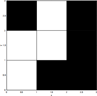
The grid and initialisation input file consists of four columns of data, each row representing an active grid point. In order, the columns are the i index of the grid point, the j index of the grid point, the initial value u at this grid point (at position xi ,yj ). They will be ordered so that Nyi + j increases with line number.
For example, the input
0 0 0.2
0 1 0.2
1 1 0.2
1 2 0.2
with input parameters Lx = 3, Ly = 3, Nx = 3 and Ny = 3 would define a computational domain (active grid cells) shown in white below:
3 Compiling
You can (and probably should) use the LAPACK library to invert matrices. This library is installed on the lab computers and on SCRTP machines (vonneumann) once you have enetered the following commands
module purge
module load intel impi imkl
Let us say your code file is named ‘prog.c’ (if not, change the filename in the compile line). The code must compile and generate no warnings when compiled with:
gcc prog.c -lmkl -liomp5 -lm
Be careful copying and pasting this command line: a script containing the compiler command is also on the website (for example if you add or remove spaces then this may prevent compilation). Please call the LAPACKE C inter-face and not LAPACK directly (because these are FORTRAN functions and the interface is not guaranteed to work the same way when compiled on different machines).
4 Test cases
Useful test cases include the trivial cases where diffusion dominates (either by using small values or switching off the nonlinear term). It would be useful to consider cases where the domain is much longer in one direction than the other. Since the number of grid points may be small, this allows 1D test cases to be run. You may wish to choose simple conditions where analytical solutions exist in linear limits. Rectangular domains allow exact solutions (via separation of variables) in the linear limit.
5 Output
The code should the value u(x, y) to a file ‘output.txt’ in five column format (ie four values per line, the time, the position indexes i and j of the grid points, then the u value) for all the active grid points (xi , yj ), at time points t = 0, tD, 2tD, ... etc. The order in which data at spatial gridpoints is output should be the same as for the input file, and all the values at each time should be in consecutive lines.
2024-02-20