Hello, dear friend, you can consult us at any time if you have any questions, add WeChat: daixieit

CS 1100 – Computer Science and Its Applications

Topic 6: Working With Text

How to Get Started

To get started, download the starter file from Canvas.

What to Turn in

You must submit your solution to Canvas by the due date.  You will be modifying a starter workbook using Microsoft Excel. When you finish the assignment, save the file and upload the .xlsx (or .xls) file to Canvas. You must name the file

LastName-FirstName .strings

where LastName is your lastname and FirstName is your full first name.

Knowledge Needed

This assignment involves the following Excel functions and techniques:

.  LAMBDA,  LET,  FIND,  LEFT,  MID,  RIGHT,  TRIM,  NUMBERVALUE,  IF,  IFERROR,  COUNTIFS, TEXT, VALUE, VLOOKUP, INDEX, MAP, MAX

.  Predefined Excel functions that you implement in simplified form:  TEXTBEFORE, TEXTAFTER, TEXTSPLIT, TAKE

.  Additional Functions:  UNIQUE, TRANSPOSE, SORT, SEQUENCE, XLOOKUP,XMATCH, FILTER.

.  3-D references, Formatting.

Keepinmindthathowyouexpresstheformulasmatters.Spreadsheetsshouldreflectanylegalchanges tothedatasuchasadding/removingrowsandchangingvaluesincells.

Allformulasshouldbedynamicwhichspillcorrectlytothedesiredcells.Youcantestyourformulaby addingordeletingrowsfromthedataset.Trytouseaminmumnumberofformulas.

It’sokaytocopyformulasacrosscolumnsaslongasyouarenotusinganyanchoring(’$’)andthereisno easywaytouseadynamicformula.

LAMBDAs in this assignment

Remember from assignment  5  and the syllabus that you need 3 items for each LAMBDA: Function Template, Convincing Argument Chat link, Formula Derivation Chat link.

1.  LAMBDA TAKECSA simulating a simple form of TAKE

2.  LAMBDA TEXTBEFORECSA simulating a simple form of TEXTBEFORE

3.  LAMBDA TEXTAFTERCSA simulating a simple form of TEXTAFTER

4.  LAMBDA exam_percentage_rule corrected.   Use  ChatGPT  to find the typo by describing the grading rules in English as a specification.   Then,  let  ChatGPT  check  the  function  against  its specification.

Problem 1 App Market Intelligence (40 points)

The sales department at aoun.com received information about a list of popular apps, which is in app market  data. The data came as a list of strings instead of using separate fields for name, downloads (ios or android), company who owns the app, and the current userbase.

The information provided a data description document with the structure of the data. It identifies every field that may appear and the layout, which specifies the order of the fields and how each is delimited. It also means that the field’sending or last delimiter may not appear within the field. The layout is:

App_Name ,IOS ,Android — Company

The red characters are the delimiters and these characters are the field names. Often in practice, you may see fields marked as .

Required means, at a minimum, that every field must be present, meaning it is not optional. Optional fields may be missing but should be represented by its delimiter. Optional field is a field that may not have a value.  Let’s look at an example.  The first line of our data is

Messenger,5,8.5  -  Facebook  <1.2B>

Suppose the data is corrupt; the app’s name is missing.  Instead the data you should look like

,5,8.5  -  Facebook  <1.2B>

Here,  is optional, there is no value but the delimiters are present (the start of the string is the first delimiter and the first comma is the second. However, its value is missing. Thus, the field’s value is the empty string.

This is an example of what’s called  syntax  and  semantics.   Syntax  concerns  the structure of the string:  e.g., is it required, how long it can be or what characters are allowed.  Semantics concerns the string’s meaning.  Here, syntax says the field has to be present, meaning delimited.  Semantics would say whether the string may be empty or have certain values. For example, you could specify the company must be a registered company.

3.  Use helper columns to the right of column I to help extract the values for columns C through I, see Figure 1. Please use column L as the first helper column for extracting the first field.

To extract the fields, write two helper functions using LAMBDA and the name manager.  Name them, TEXTBEFORECSA and TEXTAFTERCSA. The functions you are creating are modelled after Excel’s TEXTBEFORE and TEXTAFTER functions.  Please review TEXTBEFORE docu-

mentation with this link. Please also review the documentation for TEXTAFTER with this link. The TEXTBEFORECSA returns text that occurs before a given character or string.   It  is the opposite of the TEXTAFTERCSA function.

=TEXTBEFORECSA(text,delimiter)

The TEXTBEFORE function has the following arguments:

. text The text you aresearching within. Wildcard characters, such as * and ? are not allowed.

If text is an empty string, it should return the empty text "".

. delimiter The text that marks the point before which you want to extract.

The TEXTAFTERCSA function returns text that occurs after a given character or string.  It is the opposite of the TEXTBEFORECSA function.

=TEXTAFTERCSA(text,delimiter)

The TEXTAFTERCSA function has the following arguments:

. text The text you are searching within. Wildcard characters such as * and ?  are not allowed in the text.

. delimiter The text that marks the point after which you want to extract.

Use the Excel Text functions such as FIND, LEFT, RIGHT, etc., to implement the two helper functions. Ensure you can handle delimiters of any length not just single character delimiters.

You will need to use both TEXTBEFORECSA and TEXTAFTERCSA for each extracted field. If you are extracting 4 columns, you will need 8 helper columns.  Here, it is appropriate to use copying and pasting to the right unless you engage ChatGPT to help you do the iteration automatically

using the REDUCE function. For each extracted field, you control the behavior from the top three rows of the two columns.  The first row contains the delimiter.  The second row contains a comment indicating whether it is a BEFORE or AFTER column.  All the work is done by the formulas in the third row using hashtag and regular references. Here is a possible snapshot where the delimiter is a comma.

,

BEFORE                                              AFTER

=TEXTBEFORECSA(Ref_1#,Ref_2)    =TEXTAFTERCSA(Ref_1#,Ref_2)

where Ref__1# refers to a dynamic array containing the data to be processed (computed the first time by TAKECSA and thereafter by TEXTAFTERCSA. Ref_2 is a reference to a delimiter cell. This 3 by 2 matrix you copy to the right until you have extracted all columns.  Each time you copy to the right, the column coordinates shift by two columns to the right (e.g., column X becomes column Z). You must carefully initialize this process by bringing the initial data into a helper column. You also need to update the delimiters in the first row carefully.   Please  document  and develop the LAMBDA functions using a separate worksheet and follow the Function Template.

4.  Once your helper columns have the extracted fields, write a formula to copy the values from the appropriate helper column to fill in columns E through I.

5.  Format your solution as shown in Figure 1 when k=11.

Important: As a design goal, your aim should be to develop a small number of reusable formulas that you can also reuse across problems.  Points will be deducted if you have extra trailing or leading spaces in your answers.

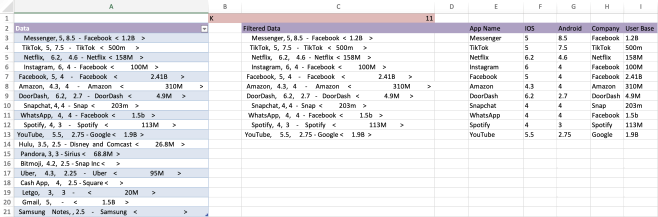
Figure 1: What your sheet for Problem 1 should look like

Problem 2    Bookstore Sales (25 points)

Important:  Insert an additional empty B column to the starter file to separate the input data from the output. Then, you can use the column names used below.

A bookstore would like to determine what kinds of books were sold on a particular day.  Data has been downloaded into a spreadsheet shown in the worksheet bookstore  sales.   The downloaded data may contain leading or trailing spaces due to a defect in the download program.  In this problem, we define the syntax of the book information using the widely used EBNF notation.  The following syntax rule describes each book:

BookTitle  "by"  AuthorName  [","  FormatCode]

BookTitle is not allowed to contain by.  AuthorName is not allowed to contain a comma.  The square brackets indicate that FormatCode is an optional field.  The presence of a comma after the AuthorName indicates that the FormatCode is in the input.  The absence of a comma after the AuthorName means that the FormatCode is absent.

1.  Transform the data in Column A into an Excel Table, rename it BookData.

2.  Create an Excel Table named BCODES for the data below to find the Type given the format code:

Format Code	Type
HC	Hardcover
PB	Paperback
EB	Ebook
AB	Audio Book

3.  In column C, extract the title of each book.

4.  In column D, extract the author of each book

5.  In column E, extract the format code of each book.  Be sure to handle codes with leading and trailing spaces.

6.  In column F, insert the type associated with the book’s format code.  Format code is an optional field, which means the format code may be missing.  If the field is missing, keep the cell empty for the Format Code column and put the value UNKNOWN in the Format column.

7.  Generate headers for columns G through J using the Format Code column in the BCODES table. Use TRANSPOSE, and SORT to create the headers from the BCODES table as well as a LOOKUP function to retrieve the book type values from BCODES.

8.  Create one formula to count (using COUNTIFS) the data for each book format in columns G through J.

9.  Find the percentage of each format sold with respect to all formats (except UNKNOWN). Store the percentage at the bottom of each column (G:J). Use one dynamic formula that is NOT duplicated.

10.  Format your solution as shown in Figure 2.

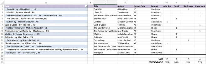
Figure 2: What your sheet for Problem 2 should look like.

next_delim_2,CHOOSECOLS(delims,2),

curr_rest_2,TAKE(acc_2,,-1),

first_2,TRIM(TEXTBEFORECSA(curr_rest_2,next_delim_2)),

rest_2,TEXTAFTERCSA(curr_rest_2,next_delim_2),

acc_3,HSTACK(acc_2,next_delim_2,  first_2,  rest_2),