MAT135 Tutorial 1 Building Mathematical Models
Hello, dear friend, you can consult us at any time if you have any questions, add WeChat: daixieit
MAT135 Tutorial 1
Building Mathematical Models
Model building is the art of selecting those aspects of a process that are relevant to the question being asked – J.H Holland
Mathematical Modelling: The Process
The mathematical modelling process is summarized in the following diagram, from SIAM’s Math Modeling guide.
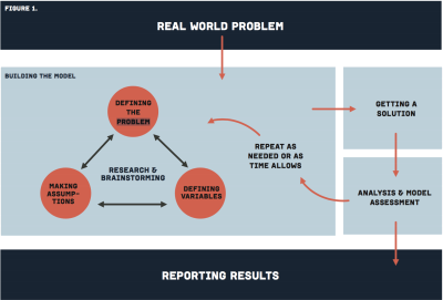
In MAT135/136, you will usually be most of the information in the ‘building the model’ box, and will focus on how to move from the given information to a solution. It is important for you to be aware of the entire mathematical modelling process, and to understand that calculus only plays a role in a small part of it.
Learning Objective
In this tutorial you will work on translating information given in words into an algebraic mathematical model. In particular, you will focus on models that involve proportionality, constant rates of change (linear models), and models built from translations of functions (e.g. trigonometric models).
All tutorials will be focused on increasing your problem solving and mathematical problem-solving skills.
Problems
1. The red curve in the graph below shows the mean monthly carbon dioxide concentration in parts per million (ppm) at the Mauna Loa Observatory in Hawaii, as a function of time t in months from January 2016 to July 2021. The black curve shows the seasonal adjusted value of CO2. In this problem, we will be working on developing a mathematical model to approximate the red curve.
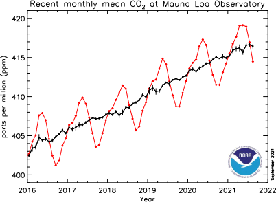
a) Approximately how much did the monthly mean CO2 increase between January 2016 and January 2021? (Note that the monthly mean is given by the red curve).
b) Find the average rate of increase of the monthly mean CO2 between January 2016 and January 2021. Be sure to include units!
c) Use the information in part b) to ind a linear function that approximates the black curve, where t is in years since beginning of 2016.
d) In preparation for the next part, graph y = sin(x), y = x, y = sin(x) + x and y = xsin(x) on the same set of axes. What do you notice?
e) The red curve may be approximated by a function of the form h(t) = f(t) + g(t), where f(t) is sinusoidal, g(t) is linear, and t is in years since beginning of 2016. Find a possible formula for h(t). (Hint: What is the approximate period of the sinusoidal function f? What is its amplitude?) If you have Geogebra, graph your function using the same scale as in the igure above.
2. In this problem we will investigate the challenge of controlling exponential growth, applied to the problem of cancer treatment. Cancer is a collection of diseases in which the patients own cells stop cooperating with the rest of their body, and decide to reproduce uncontrollably. These cells replicate to form tumour growths. The goal for most cancer treatments is to remove or kill these misbehaving cells while keeping the rest of the patient alive. For our problem, we will be assuming a hypothetical situation of a single tumour growth and one treatment for the tumour. While this is simpliied from the reality of cancer growth and treatment, the goal of this problem is to highlight how mathematical modeling of cancer, which is an active area of research that is improving patient care. If you’re interested in learning more about how these ideas are extended and applied in practice, you can learn more in the resources provided in the footnotes1 .
a) We will start by assuming that a tumour is discovered in a patient by a doctor during a routine exam. At the time of discovery, this tumour already has grown to a population of 13,500 cancer cells. Unfortunately for the patient, it is a particularly aggressive tumour, which each cell repli- cating (that is, each cell dividing into two) every two days. Create a table projecting the number of cells in the tumour for every second day over the next 14 days.
b) Given the table of values you just created, lets write down a model of what the tumour growth will be overtime (measured in days). There is a natural choice of a function for things that double regularly. Write down this function, f (t), adapted so that the number of cells at day 0 (at t = 0) is 13,500.
c) While our patient is very unlucky with his aggressive cancer, he is fortunate that his doctor can enroll him immediately in a trial for a novel, breakthrough cancer therapy. In particular, his doctor prescribes him an experimental cancer vaccine, which trains his own immune system to produce antibodies and killer t-cells that attack and kill the cancer cells. (Both companies behind the mRNA COVID vaccines, BioNTech and Moderna, are working on such experimental technol- ogy - however we are simplifying a bit on how they work for the purposes of this question).
Lets assume that once the patient produces antibodies after this vaccine, the number of antibodies begins to grow quadratically with time, following the function g(t) = 50000 * t2. However, there is a delay of 7 days after injection while the immune system responds to the shot. Lets also assume that each antibody is enough to kill exactly 1 cancer cell. Write down a piece-wise function that combines f (t) and g(t) to model the number of cancer cells left alive each day after the patient receives the vaccine. Remember to keep track of the delay in immune system response.
d) Once all cancer cells are dead, the tumour has noway of returning. Using a graph of the two parts of your function, determine whether this particular cancer vaccine is able to kill of all cancer cells present in this patient tumour. Approximately which day does this happen?
e) Catching cancer early can have a stronger efect on prognosis than the treatments given. What would happen in our hypothetical situation if the patient was delayed in receiving the vaccine by just 2 days (so that the antibody production begins on day 9 instead of day 7)? Use a graph again to answer this question.
2024-02-08