CMPUT 206 (LEC B1 Winter 2024): Assignment 2: Filters and Edge Detection
Hello, dear friend, you can consult us at any time if you have any questions, add WeChat: daixieit
CMPUT 206 (LEC B1 Winter 2024): Assignment 2: Filters and Edge Detection
Opened: Friday, 26 January 2024, 12:00 AM
Due: Friday, 9 February 2024, 11:59 PM
This assignment is worth 9% of the overall weight.
Submission guidelines:
You are provided with a single source file called A2_submission.py along with 3 images to be used as input in your code. You need to complete the five functions indicated there, one for each part. You can add any other functions or other code you want to use but they must all be in this same file.
You need to submit only the completed A2_submission.py.
Images need to be downloaded from e-class before they can be used in your code. ALL files you need are located in ONE SINGLE directory called Assignment 2 files.
Displaying Images
Please make sure that all images displayed by your submission (when run on Colab using the method described here) are large enough for the TA to make out whether they match expected outputs.
Quick help on filtering:
Skimage filters
For filtering an image with a user-defined filter, you can use scipy.signal.convolve2d (except in part I where you cannot use any built-in function that applies a filter to an image). The function scipy.signal.convolve2d is the implementation of 2D filtering in scipy. When calling it, the first argument `in1` is the input image and the second argument `in2` is the filter to be applied to the input image.
FILTERS
Part I (10%): Computing linear filters in scikit-image/python.
Read the grayscale image moon.png.
Write a function for filtering (moving window dot product) which receives an image and a kernel/filter (of arbitrary size) and outputs the filtered image which has the same size as the input image.
Using your filtering function, filter the grayscale image with the following filters and display the results.
Write your own code to implement the following filters: (You cannot use any built-in functions from any library for this.)
NOTES:
You need to appropriately pad your input image so that the output image has the same shape as the supplied input.
For the padding you can consider the constant zero padding.
Using numpy functions for padding is allowed.
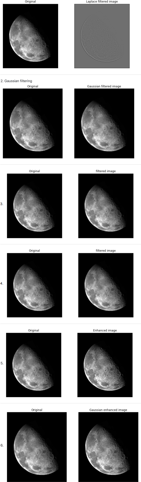
1. Laplacian Filter
2. 5x5 approximation of Gaussian filter:
[1, 4, 7, 4, 1]
[4, 16, 26, 16, 4]
(1/273) [7, 26, 41, 26, 7]
[4, 16, 26, 16, 4]
[1, 4, 7, 4, 1]
3. [0,0,0,0,0]
[0,1,0,1,0]
[0,0,0,1,0]
4. [0,0,0]
[6,0,6]
[0,0,0]
5. Compute image enhancement using a Laplacian filter and display the result. Use your result from 1.
6. Compute image enhancement using the Gaussian filter and the unsharp mask method and display the result. Use your result from 2.
Expected output for Part I:
Part II (10%): Median and Gaussian filters
Read noisy.jpg corrupted with salt and pepper noise.
Apply a median filter to remove the noise.
Apply a Gaussian filter to the same noisy image.
You can use any scikit-image functions you like. Which filter was more successful?
Expected output for Part II:

Part III (30%): An application of filtering in scikit-image: Simple image inpainting.
Write a program in scikit-image/Python to accomplish a simple image inpainting. This example and demo were shown in the lecture.
Use damage_cameraman.png and damage_mask.png.
This section highlights how image processing involves iterative algorithms.
At every iteration, your program –
(a) blurs the entire damaged image with a Gaussian smoothing filter,
(b) then, with help of the mask image, replaces only the undamaged pixels in part (a) with the undamaged pixels in the original image.
Repeat these two steps (a) and (b) a few times until all damaged pixels are infilled.
Expected output for Part III:

EDGE DETECTION
Part IV (25%): Edges
Read the grayscale image ex2.jpg.
Display the image.
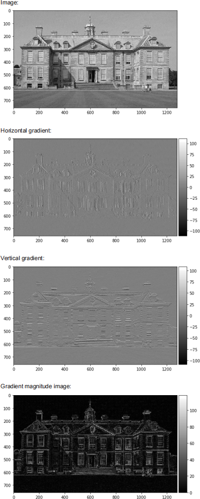
Compute the gradient of the image (both the horizontal derivative and vertical derivative) using the Sobel operators.
You can find more details about the Sobel filter in lecture notes as well as here and here. Recall that two Sobel filters are to be applied: one to compute the derivatives in vertical direction and one to compute the derivatives in horizontal direction. Obtain and display the horizontal and vertical direction derivative images. To convolve Sobel filters in python you can use the function scipy.signal.convolve2d.
The obtained horizontal and vertical derivatives should look like the second and third images shown below. Of course the output may slightly vary based on the arguments (like `mode`) that you pass to scipy.signal.convolve2d. When calling scipy.signal.convolve2d the first argument `in1` is the input image and the second argument `in2` is the filter to be applied to the input image.
Compute the gradient magnitude image by suitably combining the horizontal and the vertical derivative images. Display the gradient magnitude image. The output should look like the fourth image shown below.
Expected output for Part IV:
Part V (25%): Canny edge detector
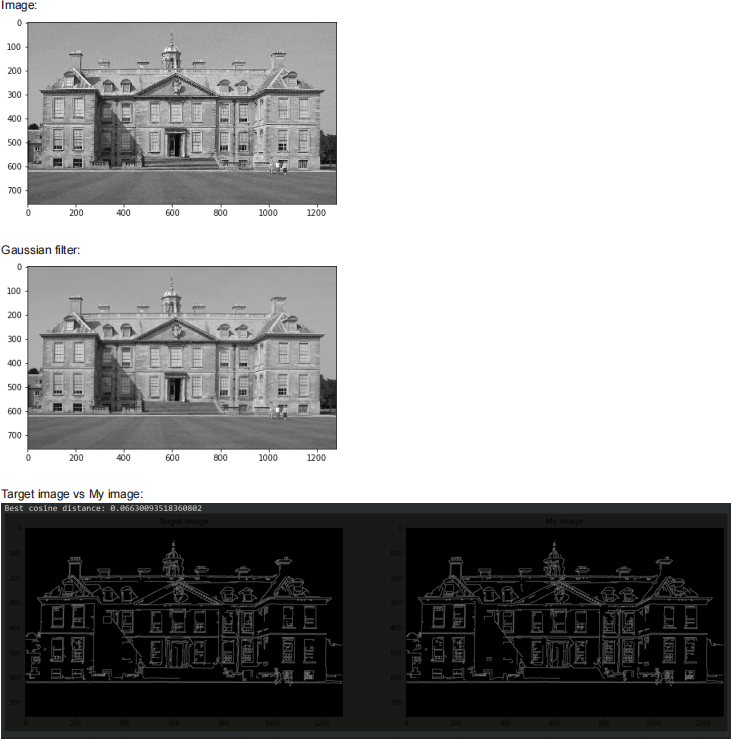
Read the grayscale image ex2.jpg and display it. Since the first step in Canny edge detection is Gaussian filtering, to understand the effect of Gaussian filtering, apply Gaussian filtering on the image and show the smoothed image. In this part to apply a Gaussian filter you can use skimage.filters.gaussian with parameters of your choice. The output may look like the second image shown below, or may look more blurred if you set the sigma argument of skimage.filters.gaussian to a large value like 10.
Canny edge detection is a multi-step algorithm and has many parameters. In this part you will be using skimage.feature.canny that implements Canny edge detection. In this link you can find a sample code for applying the algorithm.
The task is as follows. You are given an edge-detected image canny_target.jpg which is the result of applying Canny edge detection algorithm on ex2.jpg with specific values of the three parameters low_threshold, high_threshold, and sigma. Given ex2.jpg and canny_target.jpg images, in this part the goal is to find values of low_threshold, high_threshold, and sigma such that:
canny_target = canny(ex2, low_threshold, high_threshold, sigma).
To find the parameters, you should run the Canny edge detection algorithm with different combinations of the three arguments, and pick the arguments with which the output of the Canny algorithm is closest to the given canny_target.jpg. This “closeness” of resemblance can be measured using the cosine distance between the two images. To get the cosine distance between two images you can use scipy.spatial.distance.cosine. As your output, you need to plot the target Image, and the "Best" generated image, and print the minimum cosine distance. The output should look like the third and fourth images shown below. Also with the below ranges of parameters, the minimum cosine distance will be around 0.075, but any cosine distance below 0.1 is acceptable.
low_threshold in [50, 70, 90]
high_threshold in [150, 170, 190]
sigma in [1.0, 1.2, 1.4, 1.6, 1.8, 2.0, 2.2, 2.4, 2.6, 2.8]
Below you can find a pseudo-code for the task.
If the output of the Canny edge detector is all zero (i.e. all pixel values are zero), the function scipy.spatial.distance.cosine returns zero. To avoid this unwanted and trivial solution, in the below pseudo-code you can find a part that checks "np.sum(canny_output>0.0)>0.0".
S1: Read the image and the target image.
S2. Initialize best_distance to a large number, such as 1e10, and initialize the best_params array with zeros.
S3. for low_thresh in [50, 70, 90]
for high_threshold in [150, 170, 190]
for sigma in [1.0, 1.2, 1.4, 1.6, 1.8, 2.0, 2.2, 2.4, 2.6, 2.8]
canny_output = Apply the Canny method with the parameters to the image
this_dist = Compute cosine distance between canny_output image and the target image
if (this_dist < best_distance) and (np.sum(canny_output>0.0)>0.0),
best_distance = this_dist
Store current parameter values in best_params array
end-if
Expected output for Part V:
2024-02-07