Hello, dear friend, you can consult us at any time if you have any questions, add WeChat: daixieit

Student Activity Simulation with Simplified PFA Model

March 12, 2023

Abstract

This task’s goal is to simulate the learning of a set of students and predict their performance on problems according to two simplified versions of the Performance Factor Analysis (PFA) model [1] and then to discuss differences and shortcomings based on the observed behavior. You can implement the simulation in a language of your choice (Python, Matlab, R, Java, etc.). The task is to be completed in 48 hours and solutions should be submitted to [email protected]. The description here should be self-contained, and you should not need to read the reference in order to complete the task. If you feel that the problem is not fully specified, state any assumptions you need to make to solve the problem.

1 Preliminaries

We assume that a set S of students are interacting with a set Q of problems in a tutoring system. The goal of this tutoring system is for the students to learn a set of skills K. Each problem of this tutoring system is designed for one of these skills. Assignment of questions to skills are represented as 2-tuples (q, k), q ∈ Q, k ∈ K. Also, each of the problems in the system has a different level of difficulty, noted by βq for q q ∈ Q. Student activities on the problems are graded: if a student solves a problem correctly, she will receive a score of 2, and if her answer is incorrect, she will receive a score of 1 for the problem. We denote each student interaction as a 3-tuple (s, q, g), s ∈ S, q ∈ Q, g ∈ {1, 2}. We define the system’s time-steps as each individual unit of activity performed by each student: At each time-step t, students solve one problem, and thus, one 3-tuple (s, q, g) is created for student s. As students solve different problems in the system, they create sequences of these 3-tuples. Note that a student can try the same problem multiple times, in different time-steps, and have different scores in it.

We assume that students learn as they interact with the problems and that we can predict a student’s score in a problem according to her previous successes and failures in solving problems and according to problem difficulty. More specifically, if we know the number of times a student s ∈ S had succeeded in solving previous problems (had score 2), denoted by Rt−1 , and the number of times she had failed in solving previous problems (had score 1), denoted by F t−1 , then we can calculate the probability that she can solve a specific problem q at time-step t, denoted by p t sq. Performance Factor Analysis (PFA), provides a model for estimating psq based on previous student activities and problem difficulties. In the following, we see two simplified versions of PFA: No-Skill PFA and One-Skill PFA for this simulation task.

1.1 No-Skill PFA

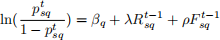
In this version of PFA, the skills are ignored in modeling student learning and predicting their performance. The assumption is that the success of student s in problem q only depends on q’s difficulty and s’s previous success and failures in q. Equation 1 shows how No-Skill PFA models the probability that at any time-step t, student s can solve a specific problem q, denoted by p t sq. Here βq represents question q’s difficulty-level, Rt−1sq shows the number of times the student s succeeded in solving the problem q previously (up to time-step t − 1), and Ft−1sq shows the number of times the student s failed in solving the problem q previously. λ and ρ parameters are success-based and failure-based learning rates for students. They measure the effect of previous success and failure in learning.

                 (1)

                       (2)

1.2 One-Skill PFA

Here, the assumption is that each question q is associated with one skill k. This assignment is represented by a binary indicator Iq,k:

                                (3)

Note that each skill k can be assigned to multiple questions. Also, we assume that the probability of student s being able to solve problem q with skill k at time-step t, a.k.a p t sq, depends on the skill that is required to solve that problem: if the student was successful in solving problems with the same skill k, including problem q. So, instead of counting the previous successes and failures for problems the q, we count the previous successes and failures for all questions j with skill k, such that both Iq,k = 1 and Ij,k = 1. The One-Skill PFA model is presented in Equation 4. Here, Rt−1sk counts the number of times student s was successful in solving any problems with skill k up to time-step t − 1 and Ft−1sk counts the number of times student s failed in solving any problems with skill k up to time-step t − 1. βq represents question q’s difficulty-level, λ and ρ parameters are success-based and failure-based learning rates for students.

                                   (4)

2 Simulation Task

You are given student activity sequences from a system in file student sequences.txt. Each row specifies a 4-tuple of student-id (s), a problem-id (q), the probability that the student succeeds in solving the problem (p t sq), and either the student’s score in that problem (ˆg) or zero. Student scores, with a probability of 1 or 0, are provided for the first activity of each student (time-step 1 for all students). For the rest of time-steps, the third and fourth values in each row (p t sq and ˆg) are equal to zero. The tuples are presented in chronological order per student-id. A set of gold-standard student activity sequences from a system is given to you in file gold standard sequences.txt. This file is formatted similarly to student sequences.txt, without the probabilities, and presents the actual scores of all student activities on problems during the whole time-period. You are also given a problem-skill assignment file, problem skill.txt. Each row in this file shows the skill that each problem belongs to, in two comma-separated numbers: problem-id q and skill-id k.

The goal of this assignment is to simulate student activity scores, given student sequences.txt and problem skill.txt, using different simulation parametrizations (defined below) and to analyze how well the simulations approximate the actual student scores (gold standard sequences.txt). For each simulation parametrization, you will fill in the zero student scores and probabilities given in student sequences.txt, and analyze the simulation results. For converting p t sq to ˆg, you can use a default value of your choice, e.g., γ = 0.5.

Here are the simulation settings to be compared:

(a) Low Learning, No-Skill PFA: in this setting you use βq = −0.001 for all q ∈ Q, λ = 0.002 and ρ = 0.001 in Equation 1.

(b) High Learning, No-Skill PFA: in this setting you use βq = −0.01, for all q ∈ Q, λ = 0.8 and ρ = 0.2 in Equation 1.

(c) Heterogeneous Learning, No-Skill PFA: in this setting you use βq = N (−0.5, 0.1)1 , λ = 0.2 and ρ = 0.05 in Equation 1.

(d) Low Learning, One-Skill PFA: in this setting you use βq = −0.001 for all q ∈ Q, λ = 0.002 and ρ = 0.001 in Equation 4.

(e) High Learning, One-Skill PFA: in this setting you use βq = −0.01, for all q ∈ Q, λ = 0.8 and ρ = 0.2 in Equation 4.

Implement the simulation in a language of your choice and use the resulting probabilities and scores to perform the analysis described next.

3 Analysis

3.1 Evaluation

Now that you have the simulated student score in each simulation setting, you can evaluate which parameter setting fits the observed scores (from gold standard sequences.txt) best.

1. How can you measure the goodness of fit to compare the different simulation settings and find out the simulation setting that is closest to the gold standard? Propose at least two different ways to evaluate the goodness of fit.

2. Calculate the results of the measures that you have suggested for each simulation setting.

3. Which simulation setting do you think is the best fit? Why?

4. Would changing the γ parameter in Equation 2 change your measure of fit results and your decision of the best setting?

3.2 Plots

For each simulation setting:

1. plot the box plot of the average of all simulated student scores on all problems in time as well as the average of all gold-standard student scores (gold standard sequences.txt) in time (all 5 setups plus the gold standard should be in the same plot). This Figure should have discrete time (time-steps) on the horizontal axis and average scores on the vertical axis. For example, if in the first time-step, student 1 works on question 1 and receives a score 2 and student 2 works on question 5 and receives score 1, the calculated average for this time-step would be  2/1+2 = 1.5. What does this plot describe? What are the findings you have from this plot?

2. plot the average student scores over all time-steps for each question for each simulated setting as well as the gold-standard. Show the 95% confidence interval error-bars for each of the averages. For example, if in the first time-step, student 1 works on question 1 and receives a score 2 and in the second time-step student 2 works on question 1 and receives score 1, the calculated average for question 1 would be 2/1+2 = 1.5. This Figure should have discrete question IDs on the horizontal axis and average scores on the vertical axis. Show 95% confidence interval error-bars for each of the settings. What does this plot describe? What are the findings you have from this plot?

3. plot the histogram of average student scores over all problems and all time-stamps per the number of time-stamps for each student. Have two plots for each setting using bin size (range) of 3 and 5 separately. For example, suppose that student 1’s sequence has 45 time stamps and the average score of this student in all questions over all 45 time-stamps is 1.5, student 2’s sequence has 46 time stamps and the average score of this student in all questions over all 46 time-stamps is 2, and student 3’s sequence has 38 time stamps and the average score of this student in all questions over all 38 time-stamps is 1. In this case, if student 1 and 2 are in the same bin, the average for their bin would be 2/1.5+2, while since student 3 will be in a separate bin, her average score will not be averaged with students 1 and 2. Show 95% confidence interval error-bars for each of the settings. What do these plots describe? What are the findings you have from these plots?

3.3 Discussion

Discuss the observed behavior.

1. Given the plots, which simulation parameter setting fits the observed scores (from gold standard sequences.txt) best in each plot setting? Why?

2. What is a possible explanation of the observed behaviors?

3. How can you further improve the fit? Discuss all the above.

4 Submission Instructions

Submit (1) your code (in a single compressed .zip or .gzip file, no executables) as well as (2) the discussion and plots from the previous sections in a pdf file to [email protected] no later than 48 hours from receiving these instructions. If you feel that the problem is not fully specified, state any assumptions you need to make to solve the problem. If you have clarifying questions, address them to [email protected].

References

[1] P. I. Pavlik Jr, H. Cen, and K. R. Koedinger. Performance factors analysis–a new alternative to knowledge tracing. Online Submission, 2009.