GGR201H5S Winter 2024 Practical Exercise 1 (Weeks 1-4): Topographic maps and glacial landforms Part iii
Hello, dear friend, you can consult us at any time if you have any questions, add WeChat: daixieit
GGR201H5S Winter 2024
Practical Exercise 1 (Weeks 1-4): Topographic maps and glacial landforms
Part (iii) Glacial landscapes and landforms in the Peterborough area, Southern Ontario
Due: Monday 5th February, 9 pm
Outline & rubric
|
Practical class |
Assignment component |
Mark |
|
January 12th |
Part (i) Analysis of Topographic Maps / Glacial Landscapes (virtual fieldwork) Section 1 – interpreting contour maps Section 2 – constructing topographic profiles Section 3 – virtual fieldwork |
6 14 20 |
|
January 19th |
Part (ii) Landscapes of glacial retreat - the Tschierva Glacier, Switzerland Section 4a – topographic profiles Section 4b – glacial landforms Section 5 – timescales of glacier retreat |
20 10 5 |
|
January 26th |
Part (iii) Glacial landforms in the Peterborough area of Southern Ontario. Section 6 – topographic profiles Section 7 – glacial landforms |
15 30 |
|
February 2nd |
Parts (i-iii) (continued) Online submission by 5th February, 9 pm |
|
|
|
Total: |
120 |
Introduction:
Part (iii) of this Practical will apply the techniques and approaches developed in Parts (i) and (ii) to
a geomorphological mapping and profiling exercise of the landscape and landforms in the
Peterborough area of Southern Ontario. This will use topographic maps produced by Natural Resources Canada and digital terrain data via Google Earth.
As a training (non-assessed) exercise in the Practical class we will explore geomorphological
mapping techniques using contour data. This will involve drawingselected geomorphological
features on a topographic map included in Appendix 1 – please ensure you have printed out Figure A2 and A3 for the practical session.
Objectives
After completion of this practical you should be able to:
1. Construct topographic profiles using contour data from Natural Resources Canada maps and compare them with profiles derived from digital terrain data (Google Earth).
2. Interpret topographic data and profile data to develop a geomorphological map.
3. Use your geomorphological maps and topographic profiles to evaluate the character of glacial landforms in the Peterborough area.
Resources (see Quercus Files/Practical Materials folder)
• Figure 5: Location Map.
• Figs 6a-c: Mapping Study Area Maps.
• Natural Resources Canada Topographic Map 31 D/8 (Peterborough): 1:50,000 scale – also available as hardcopy in the lab.
• Google Earth digital terrain data – see tutorial slides in associated pdf file (Practical 1iii Google Earth tutorial.pdf).
• Quaternary geology map of Ontario (available as a Google Earth file - goo_quaternary2021.kml
– in the Practical Materials folder).
Figure 5 identifies the mapping study areas to the east of Peterborough, Ontario. Figs 6a-c provide detailed maps of the study area as follows:
a) Normal colour reproduction of the topographic map.
b) A version of 6a which highlights the contours.
c) A lightened version of 6a which is intended for use as a base map for your geomorphological map drawing.
Instructions
Read each section below and complete the map exercises and written questions in the spaces
provided – please ensure that you print copies of Figures 6a-c and bring them to the practical. Practical 1(iii) is an individual exercise although you may discuss the work with other members of your practical group. See below for submission instructions.
Section 5
Take the time to familiarize yourself with the topography in the general area and especially in the specific mapping study area – you should take advantage of the full hardcopy and(or) PDF copies of the 31 D/8 source map and also Google Earth imagery (see instructions in the tutorial).
Section 5 exercise: Topographic profiles (15 marks)
a) Using techniques developed in Practical 1(i) and (ii), construct a topographic profile in the mapping study area to show the typical relief across an approximately E-W transect of the landscape. Ensure that your choice of profile location extends over most of the width of the map and captures one or more of the distinctive landforms in the study area, and you should also select profile start and finish points that can be identified on Google Earth, e.g. buildings, road junctions, etc. Present your profile as an attached (and labeled) diagram on the graph paper (2mm_graph_paper.pdf) that will be provided.
b) Draw your profile location on Fig. 6b.
c) Now you should generate the same topographic profile using Google Earth (see instructions in the Practical slides) in order to allow a comparison of contour-derived and digital-terrain derived data. Present the profile as a screen-grab image with an appropriate label on an attachment to your submission.
d) In the space below provide a brief description of your profiles that compares and contrasts the contour-derived and digital-terrain derived data. This should be word-processed, not hand-written (max 150 words).
Section 6
In this section you will develop a geomorphological map for the mapping study area.
Section 6 exercise: Geomorphological mapping (30 marks)
a) Using Fig. 6c as a base map, draw directly on this figure to develop a geomorphological map of the landforms on the basis of your interpretation of the contour data. You should focus on the most readily identified landforms but are free to attempt to identify and draw as many features as you can. Ensure that each feature is delimited and provided with a suitable key in the area below the mapping box. Refer to examples of geomorphological mapping discussed in Lecture 2 (and in the reference list below) for alternative mapping styles. Ensure that each map is provided with a scale and north arrow!
b) In the space below provide a brief (word-processed) description of the landforms identified in your map and in your profiles from Section 5. Account for your interpretations (i.e. how have you used topography and relief to interpret the landforms?), and include an interpretation of former ice flow directions where possible (max 300 words).
Submission instructions
Submission should be online via Quercus (Assignments / Practical 1) as a single .pdf document that combines Parts (i-iii); submit by 9 pm, Monday 5th February.
References and other useful literature
• Trenhaile (2016). Chapter 7,p.223-236.
• Clark, C.D. et al. (2009). Size and shape characteristics of drumlins, derived from a large sample, and associated scaling laws. Quaternary Science Reviews, 28: 677-692.
• Evans, D.J.A. and Twigg, D.R. (2002). The active temperate glacial landsystem: amodel based on Breidamerkurjokull and Fjallsjokull, Iceland. Quaternary Science Reviews, 21: 2143-2177.
• Livingstone, S.J. et al. (2008). Glacial geomorphology of the central sector of the last British- Irish Ice Sheet. Journal of Maps, 2008: 358-377.
• Smith, M.J. et al. (2011) Geomorphological Mapping: Methods and Applications. Elsevier.
Appendix 1: Geomorphological mapping exercise (non-assessed)
Continental glaciation advanced and retreated over North America and Europe producing many
erosionaland depositional features. Figure A1 illustrates some of the most common erosionaland depositional features associated with the passage of a continental glacier (you may also find
Trenhaile’s 2016 Chapter 7,p.218-236 helpful). The unsorted and unstratified deposits of gravel, sand, and clay form moraines, including ground and terminal moraines. Many relatively flat plains of unsorted coarse till are formed behind terminal moraines. These till plains typically have low, rolling relief, deranged drainage patterns and the following depositional features:
• Drumlins, smoothed hills made of till shaped by the ice, are oriented in the direction of the glacier's movement;
• Eskers arecurving, narrow deposits of coarse gravel left by meltwater stream deposits in tunnels beneath the ice. Often eskers end in a delta;
• Kames are small hills of poorly sorted sand and gravel that collected in depressions in the surface of a glacier.
Beyond the morainal deposits, glaciofluvial outwash plains of stratified drift feature stream
channels that are meltwater-fed, braided, and overloaded with debris deposited across the
landscape. Kettles are depressions left by melting blocks of ice that were buried in the drift and are found in both ground moraines and in outwash plains.
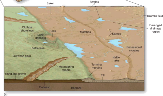
Figure A1: Common depositional landforms produced by continental glaciers (from Christophersonet al., 2013)
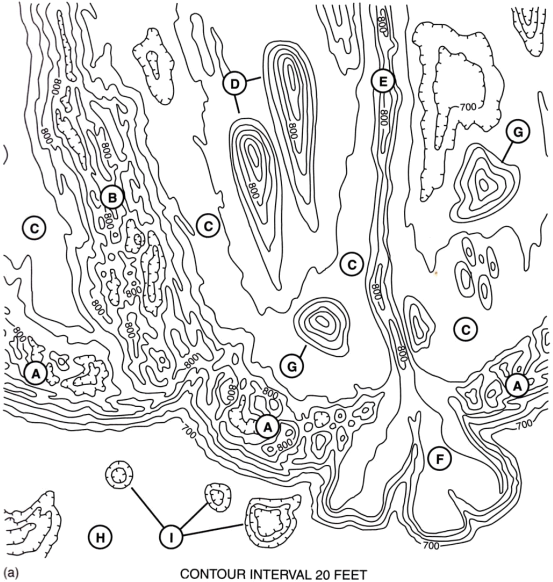
Figure A2: Contour map of a hypothetical continental (formerly) glaciated landscape
Figure A2 shows a contour map of a hypothetical landscape that has been shaped by continental glaciers.
Figure A3 (below) reproduces the hypothetical contour map from Figure A2 but with lightgrey contour coloring; this will serve as a base map for your geomorphological map (i.e. amap that identifies and delimits specific landforms) exercise to be conducted in class.
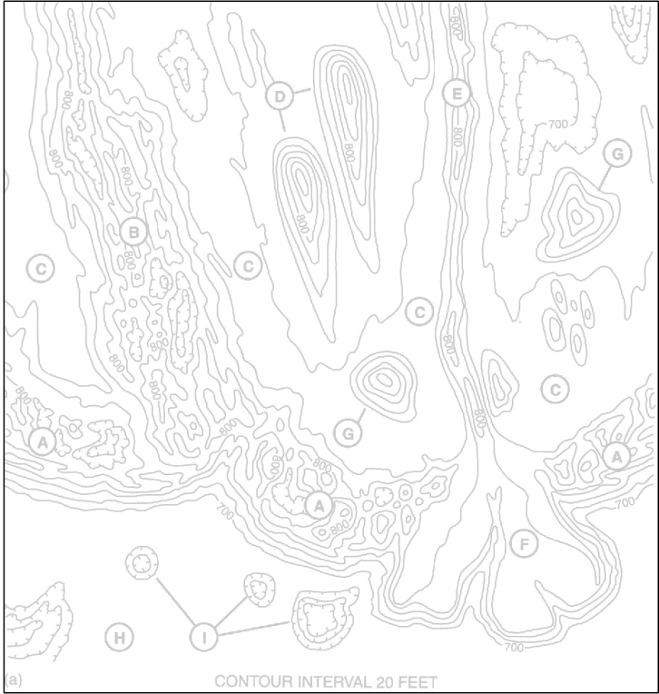
Fig A3
2024-02-07
Glacial landscapes and landforms in the Peterborough area, Southern Ontario