Goal

Implement visual servoing on Sawyer and discuss the performance of the controller. The purpose of this project is to utilize topics from Chapters 2-4 of MLS to implement closed-loop control with Sawyer.  This project is an extension of concepts from Lab 7 in Fall 2023’s EECS C106A/206A, so it’s useful to review the concepts from that lab, which can be found here. Furthermore, this project should begin to equip you with the level of expectations in 106B versus 106A. You’re encouraged to work more independently and explore robotics in a more open-ended manner.

1 Tasks

In EECS 106A, you will have implemented a feedforward and PID controller for the Sawyers and executed various trajectories.  Note that a large part of this course is developing your ability to translate course theory into working code, so we won’t be spelling out all of the theory here.

The project tasks are formally listed below.  The starter code section of this document further elaborates on the various provided files and how they all fit together.

* Developed for Spring 2024 by Kirthi Kumar, adapted from Spring 2023 by Han Nguyen.

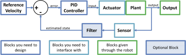
Figure 1: Block diagram of control scheme to be implemented.

1.1 Trajectories

This project fundamentally starts from having 3 different types of trajectories that you could want the robot to execute:

1.  A straight line to a goal point above an AR tag.

2.  A circle in a plane parallel to the floor (constant z value) around a goal point above an AR tag.

3.  A polygonal path in 3D space that traces straight lines between points in an arbitrary list of 3 or more goal points that are above corresponding AR tags.

You can choose your own parameters such as the height to hover above the AR tags  (we recommend somewhere around 0.2 m - 0.3 m), start point, circle radius, and trajectory duration, but make sure to clearly specify the trajectory parameters that you use in your report. Also, please explain your motivation behind choosing your particular controller.

Make sure you can execute the trajectories with MoveIt! before attempting to run them with the feedback controller you will implement.  You actually don’t have to demonstrate any results with these trajectories, but knowing they work can make you more confident for the visual servoing.

1.2 Controllers

For each controller, you will be given a desired position, velocity, and acceleration at each timestep, and your job is to design a control input in order to make the robot perform that particular desired behaviour. Please note that in this lab you must choose one controller to implement.

1.2.1    Jointspace PD Velocity Control

This will be the simplest controller you will have to implement. Here, the desired position, velocity, and acceleration,

will all be given in joint space coordinates, as θd (t), θ(˙)d (t) and θ(¨)d (t).  You will also be looking directly at the current

vector of joint angles of Sawyer’s seven joints θ(t) ∈ R7  to decide on a control input.  Recall that in driving Sawyer, we can only specify an input set of joint velocities or torques. Here, our control input will be a set of joint velocities. We will construct this in a simple proportional-derivative fashion by considering the error e(t) = θd (t) − θ(t) and its derivative. Here, θ(t) ∈ R7  is the current vector of joint angles of Sawyer’s seven joints.

1.2.2    Jointspace PD Torque Control

In jointspace torque control, our target positions, velocities and accelerations are still given in jointspace coordinates, exactly like in jointspace velocity control, but now we construct a control input of joint  torques, instead of joint ve- locities.  Once again, we incorporate error feedback in a PD fashion.  A full treatment of jointspace torque control is given in chapter 4 of the textbook.  Note that you may use either the computed torque control law from section 5.2 of chapter 4 or the PD torque control law from section 5.3.

Implementation notes:

1. You will get the jointspace inertia matrix for the robot from the KDL library.  See the respective comments in controller.py for more.

2. We have found that gravity vector returned by KDL is quite wrong.  So, we have implemented our own package to compute the gravity vector.  This is the baxter pykdl package (which contains support for Baxter and Sawyer), and you should use this to access the robot’s inertia, gravity, and coriolis terms. See the getting started section to correctly install this package, and the comments in controllers.py for exact usage.

1.2.3    Workspace Velocity Control

In workspace control, our target trajectory is no longer given as a trajectory in jointspace, but is rather given as a trajectory in workspace, gsd (t) ∈ SE(3) that we want the end effector of the robot to track.  Once again, recall that we can only supply jointspace commands to the robot.  Our strategy will be to first compute a spatial-frame workspace velocity that we would like our end effector to perform, Us (t).  This should be the velocity that will reduce the error between the current configuration of the end-effector gst (t) and the desired configuration gsd (t). Once we have such a velocity, we can use the Jacobian to come up with a joint-space velocity u ∈ R7  which we will then send to the robot as a control input.

We will compose Us  by adding up two terms, a feedforward term (which is the nominal spatial-frame velocity of the desired trajectory) and a feedback term (which will be the spatial velocity which reduces the error between the robot’s current configuration and the desired configuration at the current instant).

Recall that in implementing your trajectories, you returned the desired velocity in the form of the body-frame velocity, which happens to be the same as the spatial-frame velocity gsd  because the tool does not rotate from its starting configuration. This is exactly the feedforward term. Call this velocity Vds.

We also need to correct for the difference between the current and desired locations.  If the current frame of the

robot is gst , then the error configuration is gtd  = gst(−)1gsd.  The feedback term needs to be that velocity which reduces

the error between the t and the d frames. This is exactly ξtd , where

ξtd  = (log(gtd ))∨ .

Note that the logarithm formula and the ∨ (vee) operator are found on Page 414 and Page 41 ofMLS (page 432 and 59 in the PDF), respectively.

This feedback term velocity, however, is in the body frame.  We will need to convert it into the spatial frame using an adjoint transformation:

ξt(s)d  = Adgst ξtd.

Finally, we will put all of this together to come up with our Cartesian control law

Us  = Kpξt(s)d + Vds ,

where Kp  is a 6x6 diagonal matrix of nonnegative controller gains which you can tune.

Finally, to convert this workspace control input into a set of joint-velocities that we can send to the robot, we use the pseudo-inverse of the spatial Jacobian to get

θ(˙)(t) = J† (θ)Us (t).

Implementation notes

1.  Kp should be a diagonal matrix consisting of 6 tuneable controller gains.  Call these (Kx , Ky ,Kz , Kω1 , Kω2 , Kω3 ). The first three of these correspond to translational error in the body-frame x,y,z directions.  You can tune these differently to get different responses to errors in those three directions more-or-less independently, in a neighbourhood of the target trajectory.  The next three gains however, together multiply the angular-velocity vector of the feed-back body velocity. Note that these do not independently control rotations about three axes. Rather, they scale the different entries of the angular velocity vector.  So most likely, you want these to all be the same scalar.  However, you  can  make these angular gains higher or lower than the translational gains to prioritize maintaining the correct end-effector orientation vs the correct end-effector position.

2.  Since we will be using the Jacobian to come up with our control input, this controller is highly sensitive to the starting joint configuration of the robot.  In particular, if we start off close to certain joint-limits, the pseudo- inverse solution may try to push us toward those joint limits, preventing us from tracking the trajectory well.  So, you may need to experiment with picking different starting points to give yourself ample space in the reachable joint-space to work with.

1.2.4    Plotting controller performance

You can run the main.py script with the option --log to display plots of the performance of your controller after the trajectory is done executing. You may use these plots to tune your controller, and as part of your report. If you wish to create other types of plots from the data, feel free to change the plotting code to additionally save the data being plotted to disk for you to use later. When running with one of your custom controllers, plotting is done by the plot function in the Controller class.  Note that the plotting capabilities are not available for running trajectories with MoveIt! and will only work for your feedback controllers.

1.3 Visual Servoing

Visual servoing, also known as vision-based robot control, is when you use feedback from a vision sensor (camera) to control motion. Use one of your three feedback controllers to make Sawyer follow an AR marker with its end-effector. For example, you can make the end-effector always stay a constant offset away from the marker.

2 Deliverables

You will be expected to the deliver the following parts in your report.  Our goal with this report is to prepare you to write your final project research paper and to demonstrate that your implementation works.  Please format your report using the IEEE two-column conference template. Column suggestions do not include the figures.

1.  Methods

(a)  Explain the theory for each of the 3 controllers (workspace velocity, jointspace velocity, jointspace torque). Make sure to write the equations you derive for each controller and the reasoning behind your math.

(b)  Explain the tuning procedure for your chosen controller and state your final gain values, optional: include 1 figure per controller to supplement explanation

2.  Experimental Results

For your chosen control method:

(a)  Explain your experimental design. What experiments did you run?  Did you have a control group? If yes, what was the control group?

(b)  Plot the experimental results. Include plots with self-explanatory captions for each experiment. Your plots should compare the desired and true end-effector position and velocity as a function of time. Describe and explain any differences that you see.

(c)  Show plot(s) with captions comparing the desired and true end effector position and velocity as a function of time for visual servoing with the controller of your choice. It would be helpful to show multiple trials to ensure your results are consistent.  Why did you choose to use this controller?  How well did it perform? Describe and explain the behavior that is occurring in the plots.

3.  Applications: Give a few examples of applications where you think visual servoing can be applied.

4.  Bibliography: A bibliography section citing any resources you used. This should include any resources you used from outside of this class to help you better understand the concepts needed for this project.  Please use the IEEE citation format (https://pitt.libguides.com/citationhelp/ieee).

5.  Appendix

(a)  GitHub Link: Provide the link to your GitHub repo. We will be able to see any changes you push to your assignment repository.

(b) Videos of your implementation of visual servoing working on the robot for any one controller.  Please edit all your videos into a single video no longer than 2 minutes in runtime (you may speed your videos as long as you report your speedup factor on screen). Provide the link to your video in the report.

3    Getting Started

The lab machines you’re using already have ROS and the Sawyer robot SDK installed, but you’ll need to set up the package for Project 1.

3.1 Robot Reservations and Safety

Make sure that you have received full points on the Robot Usage Quiz. Anyone found using hardware without a full score is subject to an immediate fail for this project. We take the safety of you and your partners very seriously and want to ensure that everyone knows how to properly operate the robots.

Robots should be reserved on the robot calendars. Make sure that you do not have more than two hours reserved at a time: Sawyer Robot Calendar

3.2 Pulling starter code

Remember that groups must be composed of 2-3 students, at least one of whom must have completed EECS106A. In EECS106B, projects are going to take a while and will benefit more from collaboration compared to labs in EECS106A. Thus, we will expect you to set up a private GitHub repo for each project. As mentioned in project 0, you can find the starter code for this project in the starter repository.

3.3 Sawyer Setup

Your environment for interacting with Sawyer should be set up.  Be sure to create a folder to store all your projects for the semester. From the root of the catkin workspace, use the instructions in terminal to connect to the Sawyer.

To test that the robot is working, run the following commands:

1.  Enable the robot

2.  Test motion

3.  Start the trajectory controller (Required for MoveIt!)

4.  Check that MoveIt! works

3.4    Kinematics and Dynamics Library

For velocity and torque control, you’ll likely need the Jacobian and Manipulator Inertia Matrix. There is an existing Baxter Kinematics Dynamics Library, but we’ve modified the package to provide joint-space Coriolis and gravity vectors by exposing more of the underlying OROCOS KDL functionality as well as support for Sawyer.  These matrices returned by the kdl are slightly incorrect and may need to be tuned, for which instructions are in controllers.py.

This package is already included in your starter code.

3.5    Object Tracking with AR Markers

Create a folder called camera_info and put the file head_camera.yaml into this newly created folder.  Now make sure you’re in the directory that contains camera_info and run the following command to move this folder into a ROS subdirectory so that the camera can be set up correctly.

First you will need the AR tracking package:

The Sawyers conveniently have Logitech cameras mounted to them. Launch the AR tracking with

The AR tracking launch files publish reference frames to the tftree so you can look up the object pose with respect to any coordinate frame.  The name of the reference frame in tf is ar_marker_0 for AR marker 0.  If the script is working and the AR marker is in view of the camera you should see some output from

3.6 Starter Code

We’ve provided some starter code for you to work with, but remember that it’s just a suggestion. Feel free to deviate from it if you wish, or change it in any way you’d like.  In addition, note that the lab infrastructure has evolved a lot in the past two years.  While we have verified that the code works, remember that some things might not work perfectly, so do not assume the starter code to be ground truth. Debugging hardware/software interfaces is a useful skill that you’ll be using for years.

We have provided a bunch of files.   You  can copy in your completed  trajectories.py file from EECS  106A into the trajectories.py file here, and the most important files you should be looking at are: main.py, paths.py, controllers.py and utils.py. The others are somewhat auxiliary, or there only if you have problems.

3.6.1    Controller Implementation

The FeedForwardJointVelocityController, WorkspaceVelocityController, PDJointVelocityController,

and PDJointTorqueController inherit the Controller class.  They look at the current state of the robot and the desired state of the robot and output the control input required to move to the desired position.   Your job is to implement the step_control() function, which takes in the timestep and path object and outputs the control to follow the path.  The FeedForwardJointVelocityController has already been implemented for you as an example. It’s the same controller you saw in Lab 7 in EECS 106A (though organized a little differently).

The WorkspaceVelocityController compares the robot’s end effector position and desired end effector position to determine the control input.  Conversely, the PDJointVelocityController compares the robot’s joint values and desired joint values to generate the control input.  The PDJointTorqueController takes in the same inputs, but uses the methods we explored in lecture to generate the torque to reach the desired end effector position.

You may find the inverse_kinematics(), jacobian_pseudo_inverse(), and inertia() methods in the

baxter_pykdl package useful.  You may also find useful the set_joint_velocities() and set_joint_torques() methods in intera_interface.Limb().

Run the program using main.py.  If you set the --log flag, it will plot the end effector positions and velocities, along with their target values.

3.6.2 Visual Servoing

For visual servoing, you’ll probably want to fill out the follow_ar_tag method we’ve provided in controller.py. When following an AR tag do you need to call execute_path? Run the program using follow_ar.py. For your demo, all you need to do is demonstrate one controller working.  However, getting other controllers working to compare performance may be useful in the discussion portion of the results section.

3.6.3 Notes

A couple notes:

. You may have to edit the AR tracking launch files if you’re not using a standard wooden AR tag from the lab (those should already be on the lab desks).

.  Make sure to always source  devel/setup.bash.