1. In this problem set we extend our analysis of growth theory with optimal consump- tion by introducing the government sector.   We  do this using diferent forms of taxation.   In particular, consider the Ramsey growth model analysed in the lec- tures. Assume a government sector that every period t spends g(t) on public goods. We treat the spending requirements of the government, g(t), as exogenous.  Public goods enter directly in households utility functions such that

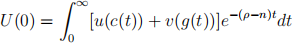
describes the representative household inter-temporal utility function, where v(.) satisies the Inada conditions.  For simplicity assume that the rate of technological progress is set to zero and depreciation rate δ is also zero.  To pay for public good provision, the government needs to raise income from taxes and must keep a per period balanced budget.

(a) Assume that g  =  g(t)  for  all t and let τ(t) denote the  lump  sum  tax  the government uses to fund of the public good.

i. Write down the individual budget constraint for this problem.

ii.  Solve for the equations of motion that describe the optimal consumption- labour and capital-labour paths.

iii.  Solve for the steady state of this economy and compare it with the version of the model in which the government sector was assumed away.  Provide an interpretation for your results.

(b)  Now assume that instead of a lump-sum the government levies a proportional tax on asset earnings, τK (t).  In this case the individual budget constraint is given by

˙(a)(t) = w(t) + (1 - τK (t))r((t)a(t) + z(t) - c(t) - na(t),

where z(t)  = τKr(t)a(t) denotes the government transfer which individuals

take as given and a(t) denotes the average asset holdings.  Since in equilibrium a(t) = a(t), the government balances its budget.

i.  Solve for the equations of motion that describe the optimal consumption- labour and capital-labour paths.

ii.  Solve for the steady state of this economy and compare it with the version of the model in which the government sector was assumed away.  Provide an interpretation for your results.

(c)  Explain what is the Ricardian Equivalence result.  How would you formalise this results using the individual’s and government’s inter temporal budget con- straint?

(d)  Now assume that instead of separable utility between private consumption and government expenditure, households’ instantaneous utility function is

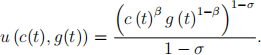
Government expenditures are inanced by lumpsum taxes τ (t).

i.  Suppose government expenditures are exogenous:  g (t)  =  g  and  govern- ment budget is balanced at each point of time, i.e., τ (t) = g (t).  Solve the decentralized equilibrium in which households take government expendi- tures as given.

ii. Does this modiication on utility function change the implications of the model, especially the Ricardian Equivalence?  Formally discuss Richardian Equivalence by considering an alternative tax plan, in which taxes are low

initially and then high later.  More speciically, τ (t) = g (t) /2 for t  < t and government debt b (t) is used to inance the gap between government expenditures and taxes. Later, taxes increase to a higher constant level to pay back the debt, i.e., τ (t) = > g for t ≥t(-) such that limt!1 b (t) = 0. Write down the government budget, i.e., dynamics of b (t). Write down the households’ maximization and resource constraint.  Discuss whether they difer from those in question (a) and the implications for the solution of the equilibrium.

iii.  Suppose that there is a social planner who choose g (t) optimally for house- holds, in addition to c (t).  How does she balance g (t) and c (t) in each period of time? Solve for the dynamic equations that characterize the op- timal path of c (t), g (t) and k (t).  Illustrate the dynamics using a phase diagram.

iv.  Suppose that the government increase g (t) fort < t from the level that the social planner sets (in question c). Discuss beneits and costs of increasing

government expenditures. Can such an increase improve welfare? Why?

(e)  Now assume that government expenditures are productive and do not directly

provide utility to households. In other words, output per capita is

f (k (t) , g (t)) = k (t)α g (t)β ,

where β 三 1, and households’ utility function is

u (c(t), g(t)) = u (c(t)) .

Furthermore, assume that government expenditures are inanced by a propor- tional tax on asset earnings, τK (t).

i.  Suppose government expenditures are exogenous:  g (t)  = g,  and govern- ment budget is balanced at each point of time, i.e., τK  (t) r (t) a (t) = g (t). Solve the decentralized equilibrium in which households take government expenditures and tax rates as given.

ii.  Does the Ricardian Equivalence hold? Why?

iii.  Suppose that there is a social planner who choose g (t) optimally for house- holds, in addition to c (t).  How does she balance g (t) and c (t) in each period of time? Solve for the dynamic equations that characterize the op- timal path of c (t), g (t) and k (t).  Illustrate the dynamics using a phase diagram.

iv.  Suppose that the government increase g (t) fort 

2.  [Extra  question:  not relavant for the exam but for people who are interested in linearization]

Consider the neoclassic growth model in the lecture with log utility, Cobb-Douglas production function, no population growth and no technology growth.

(a)  Derive the dynamic equations of c and k and compute the steady state.

(b)  Linearize the equations around the steady state.

(c)  Log-linearize the equations around the steady state:  First, take log for c and

k, and transform the equations using ˆ(c) = log c and k(ˆ) = log k; Second, linearize

the equations of ˆ(c) and k(ˆ) around the steady state of ˆ(c) and k(ˆ) .

(d)  Use the linearized or the log-linearized equations to show that the dynamic equations are saddle path stable around the steady state.  (Hint: You may try to ind the signs of the eigenvalues for the linear equations, without explicitly solving for the eigenvalues.)