Hello, dear friend, you can consult us at any time if you have any questions, add WeChat: daixieit

ELEN30012 Signals and Systems

Workshop 3: Discrete Fourier Transform [38 marks]

        Submit a report and Simulink/MATLAB files that you developed in this workshop using the LMS assign-ment link by 5pm, Friday Oct 22 (the end of Week 12). YOUR REPORT SHOULD HAVE THE ANSWERS TO ALL THE QUESTIONS AND A PHOTO OF THE EXPERIMENTS AT THAT STAGE. That is the only way that the demonstrators will be able to assess whether you have completed all the tasks or not. ANSWERS WITHOUT EXPLANATION OR MATHEMATICAL DERIVATIONS MEANS ZERO GRADE EVEN IF CORRECT. We are not interested in guessing correct answers. Ensure that you have familiarised yourself with the University rules around plagiarism before submission. You will have time in the workshops to consult with tutors around your assignment, but will need to prepare beforehand to make the best use of the available time.

        Welcome to Workshop 3 for ELEN30012 Signals and Systems. This workshop introduces to discrete Fourier transform using your home experiment kit.

1 Fast Fourier Transform (FFT)

Q: Write a MATLAB procedure that implements the fast Fourier transform (FFT).    [10 marks]

Q: Using MATLAB’s random number generator functions rand or randn, create random signals of length N. You can vary N from 10 to 106 (or higher if you want). For each N, use the FFT function that you developed earlier to compute the Fourier transform of the randomly generated signal. Record the time that it takes to compute the FFT. You can either use commands tic and toc or command timeit to measure this time accurately. Plot the recorded computational times versus N. Does this plot follow O(N log(N))? If no, why? If yes, elaborate.    [10 marks]

2 Exporting Square Wave Signal

Connect Signal Gen CH1 (DC) to Oscilloscope CH1 (DC) using a plug-to-plug jumper. In the signal generator box for CH1, dial in a square wave signal with frequency 500Hz, amplitude +1V, and offset 0V. From the menu File, click on DAQ Settings. Here, DAQ refers to data acquisition. Since the measurements can be noisy, we average a few measurements by enabling Sample Averaging in the opened dialogue window. Then, enter 10 in Number of Points. This means that each recorded output is the outcome of averaging 10 samples. The original sampling rate of the board is 375kHz. Therefore, after averaging, the sampling rate of the signal is 37.5kHz, which is more than enough for the experiments in this workshop. Select the maximum file size as 1MB. This will enable you to record roughly 100,000 samples. Click Save As Defaults. Now, from File, select Enable DAQ and then CH1. The board will record 1MB worth of samples in a location that you can specify. Please remember the location of the file for future processing. In what follows, I assume that I have recorded the outcome in a file name ch1.csv in the same directory as my MATLAB code.

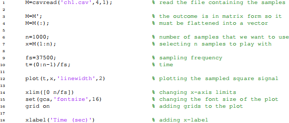
Q: Using n = 1, 000, you can observe a few cycles of the signal. Based on this, compute the frequency and amplitude of the square wave signal. Do they match what you specified on the board?    [2 marks]

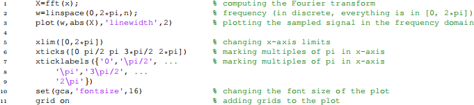
        Now, we can plot the Fourier transform the sampled signal. This can be done by the following code snippet. The following code snippet uses MATLAB’s fft function. Feel free to replace that with your own implementation of FFT from the previous section of the workshop!

Q: What’s the effect of n? What would happen if we increase n from 100 to 1,000 to 10,000 and then to 100,000? Explain why you are observing this behaviour?    [2 marks]

        Most often we use discrete information, e.g., samples of a signal, to gain some insight into continuous signals and processes. For instance, in this example, we can use the discrete Fourier transform of the signal to approximate continuous Fourier transform. The code below does this.

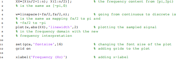
Q: Explain why the relationship depicted in the code is correct.    [6 marks]

Q: What happens if n → ∞? What should we adjust in the MATLAB code to compute the magnitude of the Fourier coefficients?    [2 marks]

3 Low Pass Filter

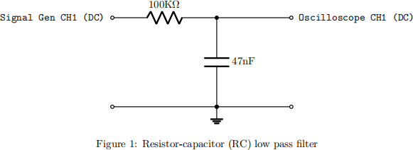
Use the components of your kit to create the circuit in Figure 1 in connection with the Labrador kit. In the signal generator box for CH1, dial in a square wave signal with frequency 500Hz, amplitude +1V, and offset 0V. Following the same procedure as before (including sample averaging) extract the output of the RC filter in another file. In what follows, the file containing the samples of the output of this circuit is named ch1_LP.csv. You can read this file and display it in MATLAB using the code below.

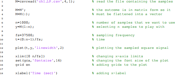
Q: Compute the frequency and amplitude of the square wave signal. Do they match those of the square wave signal?    [2 marks]

        The transfer function of the RC filter above is given by

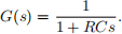
Knowing the Fourier transform of the input (you computed this earlier), you can compute the Fourier transform of the output by

We can compare this with the actual Fourier transform of the output to see if our understanding of the signals and systems correct. The following code snippet does this.

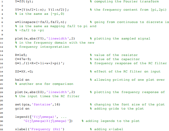
Q: Do the outputs computed two different ways match? Why?    [2 marks]

        Finally, we are going to use inverse Fourier transform to compare the output of our prediction with the actual output in time domain.

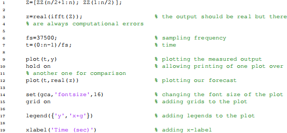
Q: Do the outputs computed two different ways match? Why?    [2 marks]