Hello, dear friend, you can consult us at any time if you have any questions, add WeChat: daixieit

MSc in CSTE: CIDA option

Advanced Java & Advanced Python Lab:

Gradient Descent Optimization

1 Introduction

In this lab we will look at a more general method for solving linear regression problems and which forms an important analysis technique in machine learning.

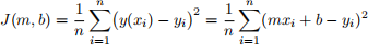
Linear regression is one of the most useful approaches for predicting a single quantitative (real-valued) variable given any number of real-valued predictors. The simplest kind of regression problem has a single predictor and a single outcome. Given a list of input values xi and output values yi , we have to fifind parameters m and b such that the linear function

is as close as possible to the observed outcome yi . We evaluate how well the pair (m, b) approximates the data by defifining a cost function. For linear regression an appropriate cost function is the mean square error.

This is an optimisation problem with some parameters (m and b) that we can tweak, and some cost function J(m, b) we want to minimise. One way of solving this problem is to use a method called gradient descent. If we imagine J(m, b) as a surface then what we are attempting to do is to fifind the lowest point on the surface. Although we don’t know where the minimum point is we can move in a direction towards it by moving downwards. The direction in which J(m, b) decreases most is given by the gradient:

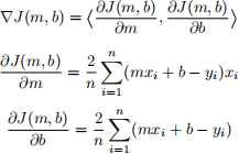
We update the (m, b) parameters in each step with

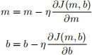
Here η is a ‘learning rate’ parameter. If we set η to a small value we approach the minimum slowly, whilst a larger value implies bigger steps and so quicker movement downhill towards the minimum but which may overshoot missing it altogether.

2 Tasks

1. Write a C++/Python/Java program which implements gradient descent algorithm for a linear regression problem based on one predictor and which takes in the value of η and the number of steps of the iteration.

2. Write a C++/Python/Java program that tests your implementation on the data set used in the class exercise. Compare the analytic solution (from the class exercise) against the gradient descent method for varying number of iteration steps, 10, 50, 100, 1000, .. and varying values of η (0.1, 0.01, 0.001, 0.0001). Use a test for convergence based on the difffferences between successive values of m and b. Take m and b to be zero initially.

3. Evaluate the ‘goodness of fifit’ by computing the r-squared test. This mea-sures the proportion of the total variance in the output (y) that can be explained by the variation in x:

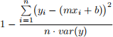
where var(y) is the variance of the y values.

4. Display your results in a table. If you can, plot the cost function J(m, b) (if using C++ or Java installing gnuplot can help here, ‘splot’ is the command to use with a fifile containing an xyz grid of points, here xyz is m, b, J(m, b)).

5. Write a report to summarise your work and fifindings.

3 Source Code and Report Requirements

Write a report to present and discuss your fifindings. The report should be no less than 1,000 words and must not exceed 2,000 words. The report can contain any number of fifigures/tables, however all fifigures/tables should be numbered and discussed. The report should include a description of the design of your solution explaining your choices. The source code should be included as an Appendix to the report.

4 Assignment Submission

The source code should be submitted electronically via the Technical Work sub-mission point by 9:30am on the 22nd October (full-time students and part-time students). The report should be submitted electronically via the TurnItInUK submission point by the prescribed deadline, for the assignment submission to be considered complete.

5 Marking

The assignment will be assessed based on the following marking scheme:

● 20% Introduction, methodology, conclusions

● 40% Source code, documentation

● 30% Analysis and discussion of the results

● 10% Report structure, presentation, references

6 References

1. https://www.cs.toronto.edu/~rgrosse/courses/csc311_f20/readings/notes_on_linear_regression.pdf

2. https://statisticsbyjim.com/regression/interpret-r-squared-regression/3. https://towardsdatascience.com/a-quick-overview-of-optimization-models-for-machine-learning-and-statistics-38e3a7d13138