STAT 4052 Homework 1
Hello, dear friend, you can consult us at any time if you have any questions, add WeChat: daixieit
STAT 4052
Homework 1
Submission policy
The homework has to be submitted electronically through Canvas before the due date indicated above.
Format
Your solution should be provided in the form of a .pdf file. Therefore, if you prepare your solutions in Microsoft Word or a similar document processing tools, you are strongly encouraged to convert your document into a .pdf file before submission.
R code
When answering questions which require R coding, DO NOT include your code in your an- swers. Report only the relevant output and your answers to the questions. All your codes should be well organized and included in the form of an appendix at the end of the document you submit.
Q1 - Read pages 29-37 of the textbook James G. et al., 2013, An introduction to statistical learning (you can find the link to it on the syllabus).
Q2 - Answer Exercise 5 on page 53.
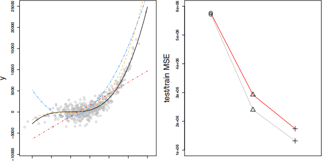
Q3 - In the plot on the left below, the data points in gray have been generated from the black curve. Whereas the red, blue and orange curves correspond to the fit obtained for the following three models:
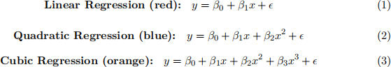
Notice that the higher the degree of the polynomial you are using the more flexible the model becomes.
The plot on the right displays the curves for the training MSEs curve (gray curve) and test MSEs curve (red curve), whereas the symbols corresponds to the values of test and training MSEs obtained for each of the models considered. In this plot, to which symbol does each model correspond to? Justify your answer.
(Hint: Review our discussion on page 3 of Handout 2 and Section 2.2.1 of the book).
Q4 - Consider the data collected in the houses.txt file available on Canvas. The dataset contains information regarding the floor area, the price, and the number of bedrooms for a sample of houses sold in a suburb of Canberra. The goal here is to assess which models among M1 and M2 below can provide the best predictions for future sales.

Notice that M2 can be easily implemented in R by specifying
sale.price ≥ bedrooms+poly(area,4)
as your model in the lm() function.
In order to compare the prediction performance of the two models, adequately estimate the test MSE using each of the following approaches:
. Validation set method by splitting 50% of the data into the training set and 50% into the val- idation set. Before splitting the data in R, set the seed using the command set.seed(1234).
. K-fold cross-validation with K = 10 using the R function cv.glm(). Also in this case, before assigning the observations to each fold, set the seed using the command set.seed(1234).
. Leave-One-Out cross-validation using the R function cv.glm().
(a) What are the estimated test MSEs you have obtained for each of the three methods above?
(b) Among M1 and M2, which model should be preferred to make future predictions?
(c) How do the estimates for the test MSE differ between the three approaches?
(d) Are the results obtained with the validation approach surprising? Justify your answer.
Q5 - Consider the following data:
y<-c(12,45,58,5,68,8,9,105,12,2,4,5,6)
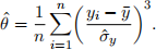
We are interested in evaluating the skewness of Y, by estimating the index of skewness, i.e.,
Before you start, it is recommended that you do a quick research on the index skewness (for instance, you may want to ask yourself: what is this index used for? How is it different from the index of kurtosis we have seen in class?).
(a) Compute the index of skewness for y using the R function skewness in the moments package. (Note: if you compute the index of skewness using the formula above, you may get different results from those given by the R function skewness, that depends on how σˆy is computed, that is, if the denominator of such estimate is n or n ≠ 1).
(b) Compute the variance of the estimator  using non-parametric bootstrap with B = 10, 000. Before drawing your bootstrap samples, set the seed using set.seed(1234).
(c) Compute the variance of the estimator using parametric bootstrap with B = 10, 000 and assuming that the observations in y are i.i.d. realizations of a Poisson random variable.
Before drawing your bootstrap samples, set the seed using set.seed(1234). (Hint: use the function rpois() to draw your samples).
(d) Looking at the results of (b) and (c), do you think that the Poisson assumption for these data is reasonable? Justify your answer.
2024-01-27