Hello, dear friend, you can consult us at any time if you have any questions, add WeChat: daixieit

Faculty of Business and Economics

2022-2023 3rd Module Examination

MFIN6002ABCDE

Spreadsheet Modelling in Finance

February 4, 2023                               2:00pm — 6:00pm

This is a take-home computer-based exam. There are 5 questions in total. Please read the instructions of each question in this exam paper carefully and finish all the questions in the Excel file.

When you answer the questions in Excel, you must include all the calculations in the worksheet.

Students can get access to internet, reference books and other teaching materials during the exam.

Students must complete the exam questions independently.

Please submit the completed Excel file on the course Moodle before 6pm. Late submission will not be accepted.

Worksheets “AMZN”, “GM”, “JPM” contain monthly data of US stocks Amazon.com, Inc., General Motors Company, and JPMorgan Chase & Co. from December 2012 to December 2022. Data are   downloaded from Yahoo!Finance.

Worksheet “ FF5 Factors” contains monthly returns data of Fama-French 5 factors (market factor “Mkt- RF”, size factor “SMB”, book-to-market factor “HML”, operating profitability factor “RMW”, and investment factor “CMA”), as well as monthly risk-free rate “RF”. Data are downloaded from Kenneth R. French’swebsite.

RMW (Robust Minus Weak) is the average return on the two robust operating profitability portfolios minus the average return on the two weak operating profitability portfolios.

CMA (Conservative Minus Aggressive) is the average return on the two conservative investment portfolios minus the average return on the two aggressive investment portfolios.

These two factors are introduced in Fama and French’s paper in the Journal of Financial Economics (2014), “A five-factor asset pricing model” .

Worksheets “ DTB4WK” and “ DBT3” contain 4-week and 3-month US Treasury bills rate in December 2022. Data are downloaded from St. Louis Fed website.

Use these data to answer Question 1 to 3.

You can add worksheets in Excel and modules in VBA whenever necessary.

Question 1 (20 points). Goto Worksheet “Q1” .

You can use Excel functions or your own VBA function/sub procedures to do calculations.

(1) (3 points) Calculate monthly log returns of three stocks from January 2013 to December 2022. Report the results in highlighted range in columns C:E.

(2) (5 points) Estimate the input parameters, including expected monthly returns, standard deviation of monthly returns, sample variance-covariance matrix and sample correlation matrix of monthly returns   of three stocks. Report the results in highlighted ranges in columns H:J.

(3) (6 points) At the beginning of 2023, you construct portfolios based on the parameters estimated in part (2).

If there are no constraints in the investment, use the analytical solutions to find the weight vector of optimal risky portfolio (P) and global minimum variance portfolio (GMVP). Report the results in highlighted ranges in columns L:N.

(4) (6 points) If short selling is not allowed, find an envelope portfolio with expected monthly return of 1%. Report the weight vector of this portfolio in range R4:R6.

Record a macro for the setting of Excel solver and name the recorded macro as “Q1_portfolio”. Save this sub procedure in VBA Module “Q1” .

Question 2 (20 points). Go to Worksheet “Q2” .

In the portfolio management, equal weight is a type of proportional measuring method that gives equal value to each stock in a portfolio, index, or index fund. In this question, we will construct an equal-weight portfolio with the three stocks (AMZN, GM, JPM) and simulate the portfolio value after 1 year.

At the beginning of 2023, the investor constructs an equal-weight portfolio (1/3 of total wealth in each stock) with AMZN, GM, and JPM. The initial investment is $100,000.

Assume that stock returns of three stocks follow Geometric Brownian motion (GBM). Discrete-time version of GBM model for log-return is

Tt →t+δt  = ln(st+δt) − ln(st ) = μδt + σε√δt,  ε~N(0,1),

and

st+δt  = st  exp(μδt + σε√δt).

At the end of each month, the investor will rebalance the portfolio such that the proportion of total wealth invested in each stock is still 1/3. Assume that this is a self-financing portfolio.

(1) (14 points) Simulate portfolio value at the end of each month from January 2023 to December 2023.

Hint: You may first simulate stock prices of AMZN, GM, JPM at the end of each month, andrecalculate the number of shares of each stock such that the proportion of total wealth invested in each stock is 1/3. You should consider the correlations between stock returns. VBA function Cholesky is given in Module “Cholesky_fn ”.

(2) (6 points) In part (1), you have simulated one time path of portfolio values in 2023. Use Data Table function to repeatedly simulate the portfolio value at the end of December 2023 for 20 times.

Please include all the calculations in the indicated area in Worksheet “Q2”. You may use Excel functions or VBA codes to generate results. You may add rows and columns in this worksheet whenever necessary.

Question 3 (25 points). Go to Worksheet “Q3” .

(1) (5 points) In columns C:E (highlighted range), construct monthly log excess returns of AMZN, GM, JPM stocks.

In columns F:K (highlighted range), calculate monthly data of Fama-French 5 factors and risk-free rates which are ready for the multivariate regressions.

(2) (5 points) Assume that three stocks follow Fama-French 5-factor model:

Rt(e) = a + β1 RM(e),t  + β2 SMBt  + β3 HMLt  + β4 RMWt  + β5 CMAt  + et

where Re  is excess return of the stock, RM(e) is market excess return, SMB is size factor, HML is book-to- market factor, RMW is operating profitability factor, CMA is investment factor.

Assume that 5 pricing factors follow normal distributions and are independent of each other. Firm- specific shock et  is independent of the pricing factors and is also normally distributed.

In range N6:R7 and N11:P18 (highlighted), use Excel functions to calculate mean and standard deviation of 5 factors, multivariate regression coefficients (a, β1, β2, β3, β4, β5 ), residual standard error and R-squared of three stocks.

Note: You should NOT use Data Analysis Toolpak to generate regression results. You must enter one formula in each cell to immediately return the desired value.

(3) (9 points) VBA functionsimfactor in Module “Q3” was discussed in the lecture. Please write a VBA functionsimfactor_new that simulates the stock price of individual stock whose log excess  return satisfies the multifactor model with up to 5 factors as described in part (2).

Note: This function should return stock price, not excess return. Please determine the arguments of this VBA function.

(4) (6 points) In range N23:P34, simulate prices of AMZN, GM and JPM month-by-month in 2023 using simfactor_new function. Feel free to estimate additional parameters.

Question 4 (20 points). Go to Worksheet “Q4” .

This question aims to use different option pricing models to calculate Facebook (NASDAQ: FB) stock option price, and implied volatility.

•    We choose a call option written on FB stock with strike price K = $175, and maturity date January 26, 2018. The option valuation date (today) is January 12, 2018. The market price of FB stock is $179.23. The market price of this option is $6.23. (Information is listed in Excel as well.)

•    Daily market data of FB stock in the past 1 year are downloaded from Yahoo!Finance and saved in Worksheet “FB” .

•    Facebook stock never paid dividends.

•    Daily 4-week Treasury Bill rates, 3-month Treasury Bill rates in the past 1 year are downloaded from St. Louis Federal Reserve website and saved in Worksheet “Tbill_FB” .

(1) (4 points) Estimate the parameters of Binomial option models for this stock and complete the input table in range B13:B20 (highlighted).

(2) (6 points) In VBA Module “Q4”, VBA function binomialCRR is given to calculate European/American option price based on CRR binomial option model.

Now in this module, write a new VBA function named binomialJR to calculate European/American option price based on JR (Jarrow and Rudd) binomial option model.

JR (Jarrow and Rudd) Binomial Tree:

JR Binomial option model is a binomial tree that is also widely used. The difference between JR and CRR  tree is the definition of (1) probability to move up, p; and (2) "up" and "down" price multipliers, u and d. Specifically,

p = 0.5,

u = exp ( (T − q − 0.5σ2)δt + σ√δt) ,

d = exp ( (T − q − 0.5σ2)δt − σ√δt)

where T, q, σ, δt have the same definition as in the CRR model.

(3) (6 points) In VBA Module “Q4”, VBA function impliedVolCRR is given to calculate implied volatility of the underlying stock based on CRR tree.

Now in this module, write a new VBA function named impliedVolJR to calculate implied volatility of the underlying stock based on JR tree.

(4) (4 points) Use CRR and JR trees to calculate this option price and implied volatility of FB stock. Report results in cells B24:B27 (highlighted).

Question 5 (20 points). Go to Worksheet “Q5” .

In this question we use Monte Carlo simulation method to price an Asian option. We assume that the underlying stock follows geometric Brownian motion (GBM) under the risk-neutral measure:

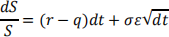
Then the stock price at time Tis given by

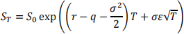
where S0  is the current stock price, Tis time to maturity, r is the continuously compounded risk-free rate,q is the continuous dividend yield, and σ is the volatility of the underlying stock.

Asian option is an example of a path-dependent option, which means that the value of the option at expiration depends upon the path by which the stock arrived at its final price. There are numerous kinds of Asian options. In this question, we value an “arithmetic average price” put option. Its terminal payoff at expiration date is

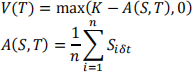
where δt = n/T is the time step in GBM model. That is, we equally divide time interval [0, T] into n subintervals. A(S, T) is arithmetic average of underlying stock price at time δt, 2δt, … , nδt (= T).

Then option price is calculated as the expected payoff at maturity T, discounted by risk-free rate over the same period, that is e−rT .

Worksheet “Q5” gives the information of an arithmetic average price put option. It will expire in 6 months. A(S, T) should be calculated as the average of stock price after 1, 2, …, 6 months. Therefore, time step δt  = 6/0.5year = 0.0833 year =  1 month.

(1) (16 points) In VBA Module “Q5”, write a sub procedure called MCMAsian that takes the following actions:

•    Read the input parameters into the sub procedure.

•    Simulate a time path of stock prices month by month from today until 6 months later (expiration date).

•    Calculate arithmetic average of stock price from the simulated time path and calculate the terminal payoff of this Asian option V(T).

•    Repeat the simulation for 100 times.

•    Write 100 simulations of the terminal payoff of the Asian option in range B20:B119.

(2) (4 points) In cell B16, calculate the Asian option value based on these 100 simulations (using risk- neutral valuation).