Hello, dear friend, you can consult us at any time if you have any questions, add WeChat: daixieit

Homework 2

Remarks:

● Students need to submit both written responses (as a pdf file) and R programs. In the written responses, when necessary, students must provide precise reference to the R program or output. Unnecessary R output must be suppressed.

● Submitting only an R program alone as your answer is insufficient. It needs to be accompanied by some verbal explanation to describe what the R program does.

● Structure your R code in a clean and succinct manner, also include sufficient comments to indicate the purpose for different parts of your code. The instructor reserves the right to deduct points for messy computer codes, especially those without any comments.

● You are strongly encouraged to use R Markdown (or knitr) to integrate R code and text response compiled to a pdf file. Submit both .Rmd (or .Rnw) file and the pdf file to Canvas.

● In all problems, you must provide your own implementation of the algorithm and attach your R code.

1. (Logistic Growth Model) The following table gives the data for the logistic growth model example in the lecture notes. Estimate the model using the Gauss-Newton approach to minimize the sum of squared error between model predictions and observed counts. And provide a scatter plot of the data imposed with the estimated growth model.

2. (Survival Analysis) The following table gives the data for the survival analysis example in the lecture notes. In this clinical trial, patients are randomized into either the treatment and control group, and their survival times were recorded. Values with parentheses are right censored. For example, (20) means the survival time exceeds 20.

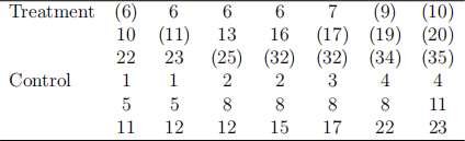
Assume the same model in the lecture notes, find the MLEs of the model parameters using the multivariate Newton’s method and Gauss-Seidel iteration, respectively. For each method, give the MLEs and draw the iteration path for each parameter. Comment on the implementation ease by comparing the two methods.

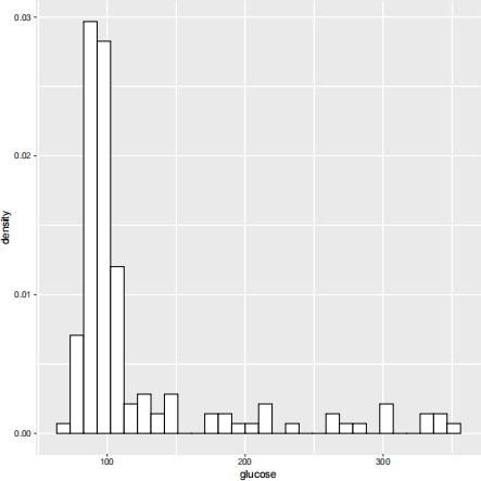
3. (Three-component normal mixture) The diabetes data set in the R package mclust contains three measurements made on 145 non-obese adult patients. For this problem, let’s focus on the glucose measurement only. You may access the data by running the following R code.

Suggested by the following relative frequency histogram, we may assume the data are i.i.d. from a three-component normal mixture model Derive the EM algorithm for finding the MLE of  i.e. give the E-step and M-step. Draw the iteration path of each parameter, and the value of the observed data log-likelihood at each iteration to demonstrate the convergence.

Next, develop the SEM algorithm for estimating the asymptotic covariance matrix of the MLEs. First provide the mathematical details of your procedure, next implement it in R, and report the the asymptotic covariance matrix in the end.

4. Consider the Baum-Welch Algorithm discussed in class. Suppose we observe a sequence of length 

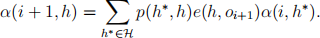
(a) Show that the following forward algorithm calculates the forward variables α(i, h).

● Initialize α(0, h) = π(h)e(h, o0).

● For i = 0, 1, . . . , n − 1, let

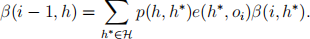
(b) Show that the following backward algorithm calculates the backward variables α(i, h).

● Initialize β(n, h) = 1.

● For i = n, n − 1, . . . , 1, let

(c) Derive the three formulas in the E-step shown in the lecture notes.

(d) First show that the complete data likelihood is

Then derive the updates in the M-step.

(e) Simulate a sequence of length 200 based on the weather data context discussed in class using true parameter value d = 0.25, w = 0.85, and s = 0.10. Then apply the Baum-Welch algorithm to the simulated data to estimate the parameter values. Plot the convergence path.