Hello, dear friend, you can consult us at any time if you have any questions, add WeChat: daixieit

SEMESTER 1 ASSESSMENT PAPER 2022/23

CENV6153

TRANSPORT MODELLING

Question 1   (Total 25 Marks)

(a) 230 residents within a city are each deciding where to go to by a birthday present for their friend. They have a choice of four locations as given in Table 1.

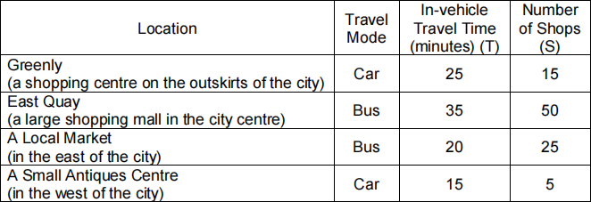
Table 1. Shopping Location Characteristics

Use a Gravity Model to estimate the number of residents choosing to shop at the Local Market. You can use the number of shops as a measure of the relative attractiveness of each location and 1/travel time(minutes) as a deterrence function. [7 marks]

(b) A shopper estimates that there is a different probability (P) of finding a suitable

present to buy in a shop at each of the four shopping locations (0.6 Greenly, 0.35 for East Quay, 0.45 for the Local Market, and 0.7 for the Antiques Centre).

The utility (U) of a shopping location is given by      U = (P*S) – 0.4T – 0.7W where W represents walking time (in minutes) to access the mode of transport, and T and S are as given in Table 1.

If the nearest bus stop (all bus routes) is a 5-minute walk, but the shopper’s car is parked only a 2-minute walk away, use a nested logit model (with the highest level   choice between travelling by car and travelling by bus) to calculate the probability of the shopper choosing East Quay. You should use a value of λ = 0.75 for any correlation parameters in your calculations. [8 marks]

(c) A larger scale survey of shopping travel within the city has identified the production- attraction trip matrices in Table 2 as representative of the [home-based] and {non-home-based} shopping trips within the city on a typical Saturday between the two main residential zones within the city (Res-1 and Res-2) and the four shopping locations.

Calculate the complete origin-destination trip matrix for shopping trips on a Saturday in the city. [10 marks]

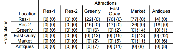
Table 2. Surveyed Trip Numbers

Question 2   (Total 25 Marks)

When construction of a new road is completed, travellers between two cities will face a choice of two routes. The Old Route is 12km long and has a maximum speed of 50km/h, the New Route is longer (17km), but has a maximum speed of 110km/h. Speed-flow curves for the two routes are shown in Figure 1.

Figure 1. Speed-Flow Curves for the Two Routes

(a) If the perceived cost of a route is equal to its travel time find the user equilibrium flow

on each route if the total number of vehicles travelling is 4096 vehicles per hour. [6 marks]

(b) Explain the difference between a user equilibrium and a system optimum assignment and show that the flows calculated in part a do not represent a system optimum assignment for this route choice. [9 marks]

(c) It has now been announced that the New Route will be a Toll Road, with a £4 toll for any vehicle wanting to use it.

If the perceived cost of a route is equal to toll(£)+travel time(minutes), show that the Method of Successive Averages does not reach a user equilibrium after 6 iterations. [10 marks]

Question 4   (Total 25 Marks)

(a) Compare the advantages of macroscopic and microscopic models and give four examples of transport studies where a microscopic model would be needed. [7 marks]

(b) An airport is considering adding an extra terminal building to increase its passenger capacity. Discuss how microscopic, macroscopic and regional scale modelling could  be used to help design the new terminal building and predict the number of additional passengers that the airport could expect. [8 marks]

(c) Surveys of all people living in a residential area have been conducted to determine levels of daily cycling trip productions for people in each of nine socio-economic groups based on age group and employment.

Table 3 gives the results of the survey where the two numbers for each group represent [total trips] and {number of people surveyed}

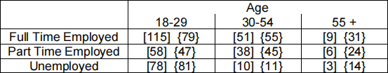
Table 3. Baseline Population and Trip Data

While the total number of people living in the residential area is not expected to change, it is expected that in the future the average age of residents will increase, and part time working will become more common.

Use Category Analysis methods to estimate the percentage change in total trips if the people living in the zone become employed as given in Table 4. [10 marks]

Table 4. Expected Age and Employment Distribution