L-questions are questions about the lecture and extra materials, H(ull)-questions are question from the book.

H2.3

What risks does a bank take if it funds long-term loans with short-term deposits?

The main risk is that interest rates will rise so that, when deposits are rolled over, the bank has to pay a higher rate of interest. The result will be a reduction in the bank’s net interest income. There is also liquidity risk.

H2.16.

Explain the moral hazard problems with deposit insurance. How can they be overcome?

Deposit insurance makes depositors less concerned about the financial health of a bank. As a result, banks maybe able to take more risk without being in danger of losing deposits. This is an example of moral hazard. (The existence of the insurance changes the behavior of the parties involved with the result that the expected payout on the insurance contract is higher.) Regulatory requirements that banks keep sufficient capital for the risks they are taking reduce their incentive to take risks. One approach (used in the U.S.) to avoiding the moral hazard problem is to make the premiums that banks have to pay for deposit insurance dependent on an assessment of the risks they are taking.

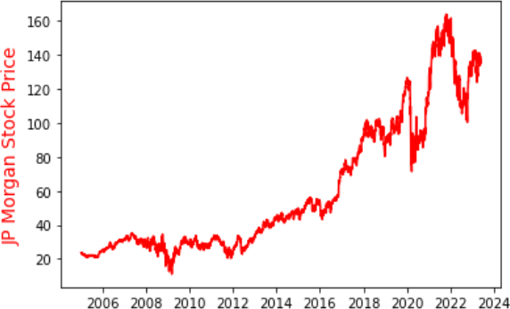
L2.1 Download the JP Morgan stock returns data from QMplus. Import the data in Python and create a line graph of the adjusted closing price. Calculate the daily log returns and create a histogram of the distribution of the log returns.

Answer

Code:

#Step 1: Import packages

import matplotlib.pyplot asplt

import numpy asnp

import pandas aspd

#Step 2: Import data

# Import CSV into DataFrame

filepath = "C:/Users/thoma/Dropbox/Queen Mary/Teaching/ECOM055 Risk Management for Banking/ECOM055_2022_23_SemC/Week 2/data2.csv"

df = pd.read_csv(filepath)

#Set index

df.set_index('Date', inplace=True)

# Convert the index to datetime type

df.index = pd.to_datetime(df.index)

print(df)

fig,ax=plt.subplots()

ax.set_ylabel("JP Morgan Stock Price",color="red",fontsize=14)

ax.plot(df["Adj Close"],color="red")

plt.show()

#Calculate the log returns

# Calculate log returns

df['Log Returns'] = np.log(df['Adj Close'] / df['Adj Close'].shift(1))

# Display the updated DataFrame

print(df)

# Display histogram of log returns

plt.hist(df['Log Returns'], bins=30, edgecolor='black')

plt.xlabel('Log Returns')

plt.ylabel('Frequency')

plt.title('Histogram of Log Returns')

plt.show()

L2.2 Calculate the 1-day 99% Value at Risk for a $1mnl JP Morgan stock portfolio, with the a. Historical method and the b. Parametric method. How to interpret the results? Explain the difference in outcomes.

Answer

Historical VaR (99%):  0.06487971593156656

Parametric VaR (99%):  0.054098074149062654

The main difference between the two methods lies in their underlying assumptions and the way they

estimate risk. The historical VaR makes no distributional assumptions and directly uses historical data, while the parametric VaR assumes a specific distribution and estimates risk based on statistical

parameters.

Code

from scipy.stats import norm

# Historical method VaR