AMSI 2024 - Bayesian Inference and Computations Lab-1
Hello, dear friend, you can consult us at any time if you have any questions, add WeChat: daixieit
Bayesian Inference and Computation
Lab 1 Exercises
These exercises provide some practice in performing basic Bayesian analyses. There is no re- quirement to do the exercises in order. Outline solutions are available in a separate file.
1) Water consumption
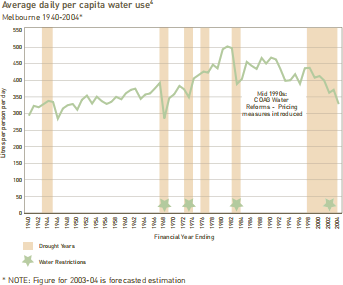
In the Melbourne average daily per capita water use analyis, we modelled the discrete observa- tions x1 ,..., xn as independent draws from a Poisson(θ) distribution. Assuming a Gamma(α,β) prior, which has a density function of

we computed the posterior as a Gamma(α +:![]() xi ,β + n) distribution.
xi ,β + n) distribution.
(a) Given that n = 65, :i xi = 24, 890 and with prior parameters α = 1,β = 0.01, compute a point estimate (i.e. the posterior mean) and a 95% central credible interval for θ. Note, you will need to compute the credible interval numerically in R (hint: use the R command qgamma).
(b) Draw a sample of size N = 500 directly from the posterior distribution (seethe R command rgamma), and obtain Monte Carlo estimates of the lower and upper values of the 95% credible interval for θ .
Repeat this 250 times, and produce a histogram for the distribution of each interval end- point. Superimpose a point corresponding to the true interval endpoints. How accurate is the Monte Carlo estimate? (R commands: hist, points).
Produce another pair of histograms, but this time use N = 5000 samples. How is the precision of the Monte Carlo estimates affected?
How many samples, N, are needed for the spread (i.e. min - max) of the Monte Carlo estimates for each interval endpoint to be less than 0.15?
(c) In lectures it was stated that the predictive distribution for a future observation, g, is
NegBin(g | α +Σi ①i , ![]() . Draw samples directly from the posterior distribution. Use these to obtain samples from the posterior predictive distribution, and plot this via a histogram. Superimpose the density of the algebraically computed negative binomial predictive distribution (R command: dnbinom). Do the distributions coincide?
. Draw samples directly from the posterior distribution. Use these to obtain samples from the posterior predictive distribution, and plot this via a histogram. Superimpose the density of the algebraically computed negative binomial predictive distribution (R command: dnbinom). Do the distributions coincide?
(d) What are the advantages/disadvantages of performing statistical analyses using the alge- braically exact approach, and the Monte Carlo approximations?
2) Estimating evolutionary fitness of tuberculosis
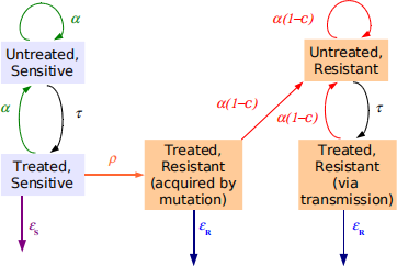
Luciani et al. (2009) developed a stochastic model (above) to estimate epidemiological param- eters relating to the development of drug resistance in mycobacterium tuberculosis. Unknown model parameters included the transmission rate (α), the marker mutation rate (μ), the mu- tation rate of drug resistance (ρ) and the transmission cost due to resistance (c). The rates of cure due to treatment for sensitive (ES ) and resistant (ER ) strains, and the detection and treatment rate (τ) are held fixed.
Samples from the posterior distribution when analysing the IS6110 marker from Cuban data can be found in the file tuberculosis. txt (the rows correspond to α , c, ρ and μ in order).
(a) Read the posterior into R (using the command read. table). Produce marginal posterior histograms of each parameter, and scatterplots of the 6 bivariate distributions (e.g. (α, c), ..., (ρ,μ)).
(b) The relative fitness of the drug-resistant strains based on the model of Luciani eta. (2009) can be expressed as

If δ = τ = εS = 0.52 and εR = 0.202 are fixed, then produce a histogram of the posterior distribution of Φ . Calculate Pr(Φ < 1), the posterior probability that Φ < 1. Is there any evidence that the resistant strain is any less evolutionarily fit than the susceptible strain? (i.e. is there any evidence that Φ < 1?)
(c) A central 95% credible interval for ρ can be estimated by discarding the lower and upper 2.5% of the posterior samples. Obtain such a 95% interval for ρ and comment on its length.
(d) A 95% credible interval is any interval for which the interval contains 95% of the poste- rior density. For example, (q0.01 , q0.96 ), where qx is the x-th quantile of a parameter, is also a 95% credible interval. As there are (in theory) an infinite number of 95% credible intervals for any parameter, convention a useful strategy is to take the shortest one.
Based on the posterior sample of length 5000, compute 250 unique 95% credible intervals for ρ, and identify the shortest. How does this compare to using the central 95% credible interval? Under what circumstances is the central 95% credible interval likely to be close to the shortest length?
3) Buffon’s Needle
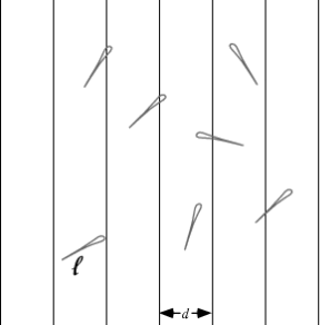
One of the most famous simulation experiments is Buffon’s Needle, designed to calculate (not very efficiently!) an estimate of π. Imagine a grid of parallel lines with spacing d, on which a needle of length ℓ ≤ d is dropped. We repeat this experiment n times and count the proportion of times,ˆ(p), that the needle intersects with a line.
The rationale behind this is that if x is the distance from the centre of the needle to the leftmost line, and if θ is the angle from the vertical, then under the assumption of random needle throwing, we would have x ∼ U(0, d), and θ ∼ U(0,π). Hence
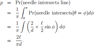
Hence, an estimate of π is ˆ(π) = ![]() .
.
(a) Produce some code to simulate the Buffon’s Needle experiment, given the lengths ℓ and d, and produce an estimate of π. Plot the estimate of π as the number of simulations, n, increases.
(b) A natural question is how tooptimise the relative sizes of ℓ and d. Consider the variability of 1/ˆ(π) .
Now nˆ(p) ∼ Bin(n,p), so Var(ˆ(p)) = p(1 − p)/n. Show that Var(1/ˆ(π)) = Var(ˆ(p)d/2ℓ) = ... =
![]()
![]() − 1)where ρ = ℓ/d. When is this minimised (for 0 ≤ ρ ≤ 1)?
− 1)where ρ = ℓ/d. When is this minimised (for 0 ≤ ρ ≤ 1)?
(c) By computing the estimate of π 1000 times and computing the standard deviation, for a range of values of ρ = ℓ/d, empirically demonstrate that your optimal value of ρ leads to the smallest variability for ˆ(π) .
There are a number of things which may (or may not!) improve the efficiency of this experiment, including:
. using a grid of rectangles or squares;
. using a cross or other shape instead of a needle
. using a needle of length greater than the grid separation.
The point is: simulation can be used to answer many interesting problems, but careful design may be needed to achieve even moderate efficiency.
2024-01-20