Hello, dear friend, you can consult us at any time if you have any questions, add WeChat: daixieit

Homework 4

AMATH 481/581

Problem 1

Consider the initial-boundary value problem

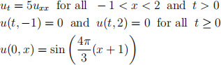
The true solution to this initial-boundary value problem is

In this problem, you will solve the PDE using the method of lines as discussed in class.  For all parts, use a second order central difference scheme with ∆x  = 0.125 (i.e., 25 total grid points) to discretize uxx. You should get a system of ODEs of the form

u′ = Au (1)

The different parts will explore different methods for solving this system.  For each part, solve from time t = 0 until time t = 0.25.

(a)  Use the forward Euler method to solve (1) with ∆t = 2−10  (i.e., 257 total time points, including t = 0 and t = 0.25).  Store your approximation of u(0.25, 0) (i.e., the value of u at t = 0.25 and x = 0) in a variable named A1.  Store the global error (that is, the maximum of the absolute values of the error at each grid point) in a variable named A2.

(b)  Use the forward Euler method to solve (1) with ∆t = 1/552 (i.e., 139 total time points, including t = 0 and t = 0.25).  Store your approximation of u(0.25, 0) (i.e., the value of u at t = 0.25 and x = 0) in a variable named A3.  Store the global error (that is, the maximum of the absolute values of the error at each grid point) in a variable named A4.

(c)  Use the backward Euler method to solve (1) with ∆t = 0.05 (i.e., 6 total time points, including t = 0 and t = 0.25).  Store your approximation of u(0.25, 0) (i.e., the value of u at t = 0.25 and x = 0) in a variable named A5.  Store the global error (that is, the maximum of the absolute values of the error at each grid point) in a variable named A6.

(d)  Use the backward Euler method to solve (1) with ∆t = 0.005 (i.e., 51 total time points, including t = 0 and t = 0.25).  Store your approximation of u(0.25, 0) (i.e., the value of u at t = 0.25 and x = 0) in a variable named A7.  Store the global error (that is, the maximum of the absolute values of the error at each grid point) in a variable named A8.

Problem 2

Consider the initial-boundary value problem

The true solution to this initial-boundary value problem is

In this problem, you will solve the PDE using the method of lines as discussed in class.  For all parts, use a second order central difference scheme with ∆x = 0.05 (i.e., 21 total grid points) to discretize uxx. You should get a system of ODEs of the form

u′ = Au + c(t)                                              (2)

where c(t) is an 19 × 1 vector. The different parts will explore different methods for solving this system. For each part, solve from time t = 0 until time t = 0.1.

(a)  Use the forward Euler method to solve (2) with ∆t = 1/550 (i.e., 56 total time points, including t = 0 and t = 0.1).  Store your approximation of u(0.1, 0.5) (i.e., the value of u at t = 0.1 and x = 0.5) in a variable named A9.  Store the global error (that is, the maximum of the absolute values of the error at each grid point) in a variable named A10.

(b)  Use the forward Euler method to solve (2) with ∆t = 0.0005 (i.e., 201 total time points, including t = 0 and t = 0.1).  Store your approximation of u(0.1, 0.5) (i.e., the value of u at t = 0.1 and x = 0.5) in a variable named A11.  Store the global error (that is, the maximum of the absolute values of the error at each grid point) in a variable named A12.

(c)  Use the trapezoidal method to solve (2) with ∆t = 0.01 (i.e., 11 total time points, including t = 0 and t = 0.1).  Store your approximation of u(0.1, 0.5) (i.e., the value of u at t = 0.1 and x = 0.5) in avariable named A13.  Store the global error (that is, the maximum of the absolute values of the error at each grid point) in a variable named A14.

(d)  Use the trapezoidal method to solve (2) with ∆t = 0.001 (i.e., 101 total time points, including t = 0 and t = 0.1).  Store your approximation of u(0.1, 0.5) (i.e., the value of u at t = 0.1 and x = 0.5) in a variable named A15.  Store the global error (that is, the maximum of the absolute values of the error at each grid point) in a variable named A16.

Problem 3 - Relevant to the written report

Consider the initial-boundary value problem

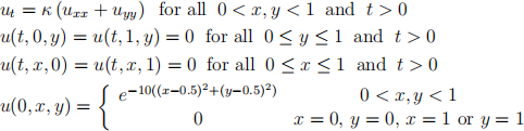
where κ = 0.1 is the diffusion coefficient (just a constant).

Note: I updated the boundary conditions for clarification. The problem is dis- continuous at the boundary at time t = 0, but this doesn’t have a substantial effect on the solution (because the heat equation smooths out discontinuities).

In this problem, you will solve the  (2 dimensional) PDE using the method of lines. For all parts, use a second order central difference scheme for both uxx  and ugg  with ∆x = ∆y = 0.1 (i.e., 11 total points in both the x and y directions). You

u′ = Au                                                     (3)

For the written report: Which of your solutions exhibit stability issues? (This should be obvious.) Suppose that your goal was just to get a rough picture of the solution at t = 0, t ≈ 1/3, t ≈ 2/3 and t = 1.  Which method do you think would be better for this purpose: Forward Euler or the Trapezoidal method? Your answer should include a sentence or two about the pros and cons of each method.