Hello, dear friend, you can consult us at any time if you have any questions, add WeChat: daixieit

SESS2019 System Design and Computing for Ships

Resistance Test Laboratory

Resistance Tests on an Arun Lifeboat Hull

Aim

To predict the naked hull effective power requirements of a full scale Arun lifeboat, over a range of speeds, based on model tests carried out in the Austin Lamont towing tank in the university.

Objectives

a) Based on the estimated effective power for the Arun Class lifeboat, figure 1, plan the speeds at which you will take resistance measurements. Conduct the experiment allowing for repeat runs in order to determine the experimental uncertainty.

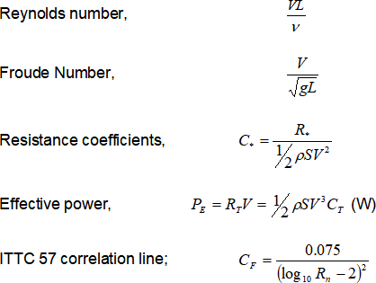
b) Calculate the skin friction coefficient, CF, at model scale (CFM) using the ITTC 57 correlation line.

c) Determine the non-dimensional residuary resistance coefficient, CR.

Background

A standard method of estimating the full-scale resistance, and hence naked hull effective power, is to carry out measurements of total resistance on a scale model of the full-scale vessel. The laboratory experiment is representative of this process and uses one of the analysis methods for extrapolating full-scale data using the ITTC 57 skin friction correlation line.

The hull model is attached via a point fixture to a tow post which allows the model freedom to pitch and heave while being towed. The tow post is attached to the carriage through a dynamometer. The dynamometer allows drag (resistance) force acting on the model to be measured. The signal can be filtered to remove some of the oscillations and the final analogue signal is fed into an analogue to digital (AtoD) converter and the digital signal is recorded in a computer via a data acquisition card. Once the signal has been calibrated the output displayed on the screen provides a measurement of the forces acting on the model.

In order to measure the drag force with as much accuracy as possible the following operations are required:

a) The dynamometer should be calibrated by applying a known load. In addition the zero level is determined when the model is stationary in calm water.

b) Where necessary, offset weights can be used to ensure that at higher towing speeds, the dynamometer does not touch the stops. The use of relieving weights ensures that the difference between resistance and offset weight lies in the measurement range and therefore the dynamometer will not touch the stops.

The model centre-line should be aligned with the tank centre-line so that the model has no yaw angle to the direction of travel. Checking the level of side force after each run will verify that the yaw angle has been set correctly. The model should be ballasted to the correct waterline in terms of total displacement and the trim angle. Both yaw and trim can have a significant influence on the levels of drag. The model is also fitted with a series of trip studs near the stem and these ensure that turbulent flow develops close to the leading edge of the model. This essentially creates a flow regime over the model that is similar to that of the ship at full scale.

It is essential to measure and record the water temperature in the towing tank so that the correct values of kinematic viscosity can be used. Note that the water in the towing tank is fresh water, whereas the full-scale vessel is assumed to operate in seawater.

The towing carriage in the Lamont tank can be driven at speeds of up to 2.5m/s, but for these tests a maximum speed of 2.2m/s is to be used. The carriage moves the model backwards to the far end of the tank prior to each test run. The model tests should be carried out in calm water. The presence of waves will alter the measured resistance and hence alter the prediction of the power required at full scale. It is therefore necessary to wait before commencing each run until the water in the tank is quiescent. Once a test run is started, the carriage will accelerate to the pre-set steady speed, it then holds this steady speed over a measured distance of approximately 10m, after which it is decelerated to rest. The measurement of the force is usually taken as a mean value over the steady-speed region of the run. It is also prudent to examine the complete measured signal as this can provide insight into the quality of the data and indicate any problems that may develop.

Experimental procedure

1) Measure and record the tank water temperature and read-off the corresponding value of kinematic viscosity from Table 2.

2) Weigh the Arun lifeboat model and tow fitting and therefore calculate the ballast weight required to provide the correct displacement. This should be within 1% of the total displacement required.

3) Switch on the computer and run the data acquisition program. Ensure that the signal amplifiers are switched on and confirm that the data acquisition program is receiving signals from the correct transducers (i.e. drag and side force). Further instruction on the data acquisition program will be provided by the lab supervisor.

4) Calibrate the drag and side force dynamometers by applying known weights to the different load cells (0N, 2.5N & 5N are typical values to use). Further instruction will be provided on how to accomplish this by the lab supervisor.

5) Carry out a series of towing tests for the required range of speeds. Ensure that the water is quiescent before the start of each run. Acquire data using the data acquisition program whilst the model is travelling through the steady speed region of the run. The carriage control software logs the speed of the run. By estimating the time the model should take to go through the steady speed section you will be able to stop the data recording just before the model leaves the steady speed section (and starts to decelerate). Obviously, any part of the record taken outside the steady speed section will have to be truncated to give an accurate level of the constant force required to propel the model at the requested steady speed. At the end of the run, note the mean levels of the forces. Furthermore, you will be able to determine if, and how much, offset weight is required for the higher speed runs.

6) Use the interval between runs to examine the full data records from the previous run and also keep an ongoing plot of CTM against Fn. Both of these actions will allow you to verify the quality of the data, and foresee any problems that may develop.

7) You should repeat any runs where the data appears to be suspect (and note the reason for this choice). Furthermore, you should repeat one of the runs at least once (or more if time permits) to determine the levels of repeatability of the experiment. This is particularly important as you should comment on the implications of the experimental variation on the calculations of effective power for the full scale ship.

Laboratory report

You should keep your report clear and concise, and adopt an accepted technical writing style. The report should include clear statements of the aim and objectives. You should briefly present the methodology, although a word-for-word transcription of the supplied guidance is not required; a critique on the practicalities and challenges involved in the procedure may be appropriate. You should include a presentation of your results and analysis in graphical forms, clearly showing the workings and written explanations of the progression from one stage of the analysis to the next. In particular, you should include a plot of the raw data (R_TM v Speed), a plot showing CTM, CRM and CFM. It would also be appropriate to comment on the general shape of these plots and the relative contributions the different physical components of drag to the total drag. You should also provide analysis to indicate the effects of experimental variation on these predictions. Your report should finish with a summary, drawing together salient points and conclusion of the tests and the resulting predictions. You are also encouraged to supplement your understanding and intellectual critique of this laboratory by using standard naval architecture texts.

Relevant Data

1 knot = 0.5144m/s

Model Data

Wetted surface area,         Sm = 0.423m²

Waterline length,   LWL = 1.168m

Weight of towing post and guides 1.32 kg

Model and tow fitting weight (measured) kg

Ballast weight (calculated) kg 

Total displaced weight 13.80 kg

Ship Data

Wetted surface area m²

Waterline length 14.02 m

Total displaced weight kg

Fluid Data

Tank water temperature ^OC

Use standard values for fresh and seawater density.

Useful Data and Formulae

      Table 2: Values of kinematic viscosity for fresh water at different temperatures

(Note: values in table have been multiplied by 10⁶.)

Kinematic viscosity for salt water at 15^OC: VSW=1.18831´10^-6

Example Results

Table 3: Model resistance results

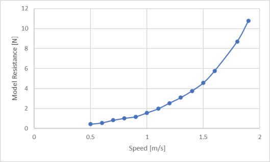
Figure 1: Model Resistance against speed