Hello, dear friend, you can consult us at any time if you have any questions, add WeChat: daixieit

PHYS2041 - Quantum Physics

Laboratory – Photoelectric Effect

Warning: This experiment uses spectral lamps that emit ultraviolet radiation. Please note the following precaution:

● The mercury spectral lamps emit UV radiation. Do not stare into the lamp. Avoid expo-sure where possible by switching the lamp off or facing it towards the wall when not in use. Students and staff must wear safety glasses during the experiment. The rims of the glasses must be cleaned using the wipes provided before and after use.

Further risk assessments are given in the appendix - please read these before starting your experiment.

1 Introduction

In 1887, Hertz discovered that a circuit containing a capacitor would conduct electricity when one of the capacitor plates is illuminated with light of sufficiently short wavelength. This phenomenon conflicted with the accepted knowledge about light at the time. In 1905, Einstein refined Planck’s proposal that electromagnetic radiation was energy quantised. He stated that these quanta, now called photons, interact individually with the electrons of the illuminated surface.

This process is called the photoelectric effect, and is complicated by two factors: (1) the presence of the minimum amount of energy required to free an electron from the surface, called the work function and (2) that the electrons in a material do not have a single kinetic energy, but rather a distribution of kinetic energies.

In this experiment you will investigate the intensity and frequency dependence of the maximum kinetic energy of the photoelectrons (electrons ejected through the absorption of light). This will allow you to determine Planck’s constant. You will also experimentally characterise the photoelectron kinetic energy distribution. The two experiments use separate sets of equipment which are shared with another group – you can expect to have one week on each set of equipment.

2 Background

The electric potential associated with a charged ion is the familiar 1/r Coulomb attraction. When several of these are placed side by side, the result is a well with the rippled bottom, as shown in Figure 1. Following this model, we can represent the interior of a solid as a square well with rounded edges. Generally, electrons like to inhabit the lowest available energy states and fill the well up to a certain level, the Fermi level Ef, rather like water filling a bath tub (see Figure 2). This is called the Fermi gas model, with the electrons in this case forming the “gas”. At zero temperature, only energy levels below Ef will be occupied, as if the surface of the “water” were flat.

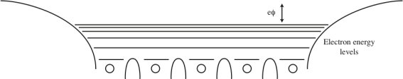
Figure 1: Energy levels of many charged ions.

Figure 2: Rounded square well potential.

2.1 Maximum photoelectron kinetic energy

Consider a photon of energy hν absorbed by an electron in a metal, causing the electron to be ejected. The maximum kinetic energy of the ejected electron is

where h is Planck’s constant, ν is the frequency of the photon, e is the charge on an electron, and φ is the work function, measured in volts.

We can measure Kmax by applying an external electric field which opposes the electron motion, and adjusting it until no electrons can reach the collecting electrode. This stopping (cut-off) potential will be linearly related to the wave number of the incident radiation and independent of its intensity

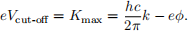
The wave number is k = 2π/λ. It is also called the spatial frequency; instead of cycles per second, it is cycles per metre. From this relationship we can see that a plot of Vcut-off versus k will yield a straight line with slope hc/2πe, and thus allows Planck’s constant h to be determined. At non-zero temperatures, the surface of the Fermi sea will not be flat, with some electrons thermally excited to energy levels above the Fermi Level. So long as a consistent method is used to determine the stopping voltage, this should have no effect on the slope and hence the determination of Planck’s constant. It can, however, affect the work function φ determined for the metal.

2.2 Photoelectron kinetic energy distribution

The emitted electron kinetic energy distribution, termed the electron energy distribution function, is denoted N(K, ν). The quantity N(K, ν)dK is therefore the probability of finding an electron with kinetic energy in the range K → K + dK. This is practically obtained by measuring the dependence of the current i(V, ν) on the retarding voltage V , with incident light frequency ν. The quantity i(V, ν) is called the current-voltage characteristic curve, and it related to N(K, ν) in ideal circumstances through the integral

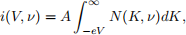
where A is a constant dependent on the incident light intensity and the electron collection efficiency, and e is the charge of an electron.

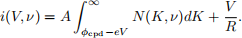
Two technical imperfections significantly affect the observed current-voltage characteristic curve. Firstly, the anode and cathode plates do not form an ideal capacitor, having a large but not infinite resistance R. This causes current leakage from the anode to the cathode. Secondly, connecting the anode to the cathode results in a contact potential difference φcpd. Essentially, there is a voltage between the plates even in the absence of the battery. This phenomenon is described in more detail in the Appendix. Together, you should see that these imperfections change  the relationship between N(K, ν) and i(V, ν) to

The result is that the characteristic curve is blurred out due to the finite temperature, tilted due to charge leakage, and shifted along the voltage axis due to the contact potential difference, as shown in Figure 3. N(K, ν) can be determined by taking the derivative of the characteristic curve with respect to the retarding voltage V

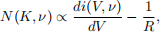
where K = φcpd − eV is the minimum kinetic energy of an ejected electron capable of reaching the cathode. Note, N(K, ν) is a probability density, therefore the absolute value can be determined by setting its integral over all energies to unity.

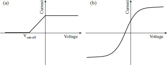
Figure 3: Sketch of the current-voltage characteristic curve for (a) the ideal case, and (b) including finite temperature, current leakage, and contact potential difference.

2.3 Exercises

Include the details of these exercises in the relevant sections of your report:

1. Carefully explain the origin of the relationship between N(K, ν) and i(V, ν) in Equation 3, highlighting why it makes intuitive sense. Reference [1] may help.

2. Research how to calculate a derivative of numerical data. Identify some of the challenges associated with this, and briefly outline how you might minimise numerical errors. Reference [3] may be useful.

3 The experiments

An accurate method to determine the cut-off voltage is critical to the success of photoelectric experiments. We will investigate two methods in this experiment as depicted in Figure 4.

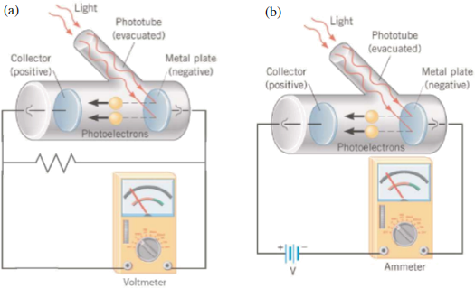
Figure 4: Photoelectric experiment configurations using (a) direct voltage measurement, and (b) traditional current measurement.

Direct voltage method

This method uses the photoelectric current itself to charge the anode and create the retarding potential. The photoelectric current will stop when the stopping potential is reached, at which time the voltage between the anode and the cathode will equal the stopping potential Vcut-off. This Vcut-off can then be measured across a resistor connected between anode and cathode. An ultra-high resistance is required to negate charge leakage from the anode. This is shown in Figure 4a.

Traditional current method

This method measures the current flowing through the photoelectric circuit as shown in Figure 4b. A retarding potential applied to the collector (cathode) repels photoelectrons, with current ceasing once the potential reaches the stopping potential Vcut-off. This approach offers the benefit of yielding a current-voltage characteristic curve for the system which, among other things, provides information about the kinetic energy distribution of the emitted photoelectrons. However, as you will see, it also introduces two types of difficulties, the most important being that the circuit couples the anode and cathode. As a result of this, the contact potential difference must be taken into account.

Note: There are separate sets of equipment for each of the two experiments. You will have exclusive access to each equipment set for only one week of the two weeks allocated for the experiments. Please negotiate with other groups allocated to this experiment to decide which week you will use each equipment set.

3.1 Experiment 1: Properties of stopping voltage and Planck’s constant

In this experiment, you will investigate both the intensity and frequency dependence of the maximum photoelec-tron kinetic energy, as well as determining Planck’s constant, h. In Part A you will select two spectral lines from a mercury light source and investigate the maximum energy of the photoelectrons as a function of the intensity. In Part B you will select different spectral lines and investigate the maximum energy of the photoelectrons as a function of the frequency of the light. You will then use this data to calculate h.

The equipment to be used in this experiment is shown in Figure 5. There are two different sets of equipment for Experiment 1. Either can be used for performing the measurements described here.

Using equipment set (a)

The equipment set in Figure 5a consists of a mercury lamp with a dispersing element – the spectral lines from the lamp are spatially separated and the detector arm is rotated to make measurements for different spectral lines. Since the green and yellow spectral lines are very close together, there is a corresponding coloured filter that should be placed over the detector before taking measurements using these lines. There is also a set of variable transmission filters for controlling the intensity of the light source. With this equipment, the output from the detector is a direct measurement of the stopping voltage.

Note: Before each stopping potential measurement you should press the PUSH TO ZERO button on the side panel of the h/e apparatus to discharge any accumulated potential in the unit’s electronics. This will ensure the apparatus records only the potential of the light you are measuring. Note that the output voltage will drift with the absence of light on the photodiode.

Using equipment set (b)

The second equipment set, shown in Figure 5b differs slightly in that the mercury emission lines are isolated spectrally by the use of filters on a filter wheel in front of the detector. Changing the size of the aperture in front of the detector controls the intensity of the light arriving at the detector. With this equipment you must vary the voltage (in the range -4.5 V to 0 V) until the current on the ammeter is zero (use a range of 10⁻¹³ A) – this then gives the stopping voltage.

Note: Before starting your measurements disconnect the cables from the back panel of the apparatus, press the SIGNAL button to “in” and adjust the CURRENT ADJUST knob until the current reads zero. Then set the SIGNAL button to the “out” position to start the measurements.

Figure 5: Equipment sets for Experiment 1.

Your tasks

Switch on the light source for your equipment set and allow at least 10 minutes for the lamp to warm up before measurements are taken. Remember to wear the safety glasses at all times while the lamp is on.

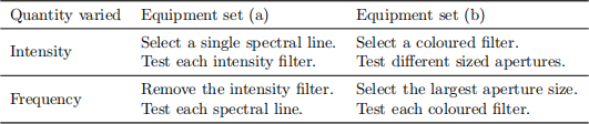
There are two parts to this experiment: measuring how the stopping voltage varies with the intensity of light, and measuring how the stopping voltage varies with the frequency of light. The quantities to change and measure and summarised in the Table 1 for each experimental apparatus.

Table 1: Parameters to fix and change. The stopping voltage should be recorded for each experiment.

Note: For apparatus (a) it is important that the spectral line hits the detector for all measurements during the experiment, so take care not to misalign the system, and check the alignment regularly throughout your measurements.

You should address the following tasks in the relevant sections of your report:

1. Describe the effect of using different intensities of the same coloured light on the stopping potential and thus the maximum energy of the photoelectrons.

2. Describe the effect that different colours of light have on the stopping potential and thus the maximum energy of the photoelectrons.

3. Defend whether this experiment supports a wave or a quantum model of light based on your results.

4. Find the exact frequencies and wavelengths of the spectral lines you used and plot the measured stopping potential values against light frequency for all sets of measurements.

5. Fit the plots according to Equation 2, extracting values for slopes and intercepts. Hence determine h and φ. Look up some values of work functions for typical metals. Is it likely that the detector material is a simple metal?

3.2 Experiment 2: Current-voltage curve and kinetic energy distribution

In this experiment you will make traditional measurements of the stopping potential using a retarding voltage applied to the anode, as shown in Figure 4b.

Apparatus

The measuring apparatus, shown in Figure 6, consists of a photodiode detector which is in series with a sensitive picoammeter. The voltage across this combination is measured with a digital voltmeter as the photodiode is illuminated using a mercury lamp. The photodiode is illuminated with light from a lamp, and has a set of narrow-band colour filters to allow you to control the frequency of incident light.

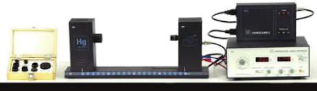
Figure 6: Experimental apparatus for Experiment 2.

Switch the lamp on and allow it to warm up for at least 20 minutes. Ensure you wear the supplied safety glasses to minimise exposure to UV radiation.

Initially use a voltage setting of -2 V to +30 V and a current range setting of 10⁻¹¹ A. You will need to perform a calibration by pressing the PHOTOTUBE SIGNAL button in to CALIBRATION and adjusting the CURRENT CALIBRATION until the current is zero.

Your tasks

You should take measurements of the current voltage characteristic curve for at least two different filters. In order to take a good derivative, you will need to take many current reading for closely spaced voltages, especially around the cut-off region. Have a play with the voltage, and try to determine roughly where the cut-off voltage is. We recommend taking readings over a range of about 4 V on either side of the cut-off if possible, with perhaps a total of 80 measurements.

From the current voltage characteristic curve you should be able to determine both the electron kinetic energy distribution and the resistance R of the capacitor formed by anode and cathode. Plot the electron kinetic energy distributions obtained for each filter setting. Would you expect them to be of this form? What differences do you observe for the different filters?

References

[1] Apker, L., Taft, E. & Dickey, J. (1948). Photoelectric emission and contact potentials of semiconductors. Physical Review, 74 (10), 1462-1474. doi:10.1103/PhysRev.74.1462

[A useful primary source for the theory of the photoelectric effect. In particular, Section II Theory of retarding potential measurements is relevant.]

[2] Knight, R.D. (2017). Quantization. In Physics for scientists and engineers: A strategic approach with modern physics (4th ed., pp. 1107-1139). Boston, Massachusetts: Pearson.

[Sections 38.1 The photoelectric effect and 38.2 Einstein’s explanation introduce the photoelectric effect and the concept of quantisation quite well.]

[3] Sauer, T. (2018). Numerical differentiation and integration. In Numerical analysis (3rd ed., pp. 253-292). Hoboken, New Jersey: Pearson.

[Of particular relevance are Sections 5.5.1 Finite difference formulas and 5.1.2 Rounding error.]

Revised: September 14, 2020

Appendix: Contact potential difference

Connecting the anode and cathode in a circuit, and including a battery introduces significant complexity. When the anode and cathode are uncharged and not connected to each other they look like two isolated bath tubs with the bath tub rim at the same potential (V = 0) as shown in Figure 7.

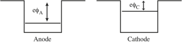
Figure 7: Isolated potentials.

When we connect these two metals together, some of the electrons from one will flow into the other, charging it negatively, and equalising the two Fermi levels, and thus altering its potential as shown in Figure 8. The flow will be very small and will cease when the two Fermi levels are at the same potential. This is what gives rise to the “contact potential”.

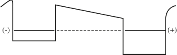
Figure 8: Contact potential.

If we connect a battery (source of emf) between these two metals, the Fermi levels are further separated by the amount of the battery potential, see Figure 9.

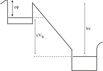
Figure 9: Biased potentials.