Econ 659 - Problem 3
Hello, dear friend, you can consult us at any time if you have any questions, add WeChat: daixieit
Econ 659 - Problem 3
Fall 2021
Subject: Sequential Market Equilibrium and Arrow-Debreu Equilibrium
In this problem set you will use Matlab to compute sequential market equilibria for the economy studied in Problem set # 1. Note that this means that we look at the simpler case where there is only ONE good. We want to compare sequential market equilibria with the contingent market equilibria of the previous problem set. Read pages 37-40 and Sections 8 and 9 in MQ. I have also posted MM Lecture 7 on Blackboard which introduces sequential markets which you will find useful. As I point out in the notes you will need to modify the budget equations of the agents to allow for their initial ownership shares of equity. In Problem D you do not use Matlab: you solve the equations defining a Pareto optimum or an AD equilibrium analytically.
Consider the economy of Problem set #1 with 3 agents (i = 1, 2, 3), one good and two dates (t = 0, 1) with 4 possible states at date 1. When applicable in each of the problems that follow, use the following notation: for agent i let  = holding of bond ,
  = share of equity of firm 1,
  = share of equity of firm 2; let
  = (0, 0) (initial share holdings of agent 3),
  = (1, 0) (initial share holdings of agent 1),
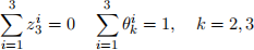
  = (0, 1) (initial share holdings of agent 2). In a sequential market equilibrium we must have
C. Sequential Market Equilibrium
(1) Let pr(k, i) = 1/2 for all k and i,  = 0 for all i and α = 2, b1 = b2 = 500, b3 = 1000 : suppose also that the only traded security is the riskless bond with payoff (1, 1, 1, 1) and that agents have no initial holdings of the bond (agents do not inherit debts from the past and the bond is in zero net supply).
(a) Assume, as in question 1 of B, that there is no risk: ε1 = ε2 = 0. Calculate the SM equilibrium. Compare the allocation and the interest rate r with that of the AD equilibrium obtained in question 1 of B (of course in the AD equilibrium we mean the interest rate
implied by the AD price of the income stream (1, 1, 1, 1)). Explain the intuition of the result.
(b) Suppose now that we add risk to the economy, as in question 2 of B, by setting e1 = 100, e2 = 200. Calculate the SM equilibrium. Compare the interest rate with the interest rate in (a) (here you are comparing the effect of adding risk with the same market structure). Also compare the interest rate with that obtained in question 2 of B (here you are comparing how agents cope with the same risk with two different market structures). What do agents try to do when they can only use the bond to cope with date 1 risk? Does this help you in explaining why you find that
? You may find it easier to understand what’s going on by examining what happens to the ‘bond price’ rather than the ‘interest rate’.
(2) We continue to assume that pr(k, i) = 1/2 for all k and i,  = 0 for all i and α = 2, e1 = 100, e2 = 200 (as in question 2 of B). But we assume that two new securities are added by letting agents 1 and 2 issue ownership shares to their (firms) income streams: thus there are three securities: the riskless bond in zero net supply, the equity of firm 1 whose payoff is the date 1 endowment of agent 1, and the equity of firm 2 whose payoff is the date 1 endowment of agent 2: the latter two securities are both in positive net supply. Agent 1 (2) is full initial owner of his equity and can sell part of it to the other agents on the equity market.
(a) Are the financial markets complete?
(b) Find the SM equilibrium and compare it to the AD equilibrium found in question 2 of B. Is there a surprise here?
(c) Use question 2(b) of B to explain the result found in (b).
(d) Note that in the SM equilibrium that you have just found in (b) none of the agents use the bond. It can be shown that this comes from the fact that the three agents have the same constant-relative-risk-aversion. If there were trade on the bond, one agent would have to leverage his portfolio and would be in a relatively riskier position than the others. Suppose that we keep all the parameters the same except for the coefficient
of agent 3. Compute the SM equilibrium for
= 500,
(3) Let’s return to the case where = 0 for all i, and lets continue to assume that agents 1 and 2 face idiosyncratic shocks, e1 = 100, e2 = 200. Suppose now that the agents have different assessments of the probabilities of success of the firms given by

Suppose that the securities are the riskless bond and the equities of the two firms. Find the SM equilibrium and compare it to the AD equilibrium of the same economy.
(4) Suppose you keep the economy the same as in the previous question, except that we add a fourth security with payoff stream (0, 0, 0, 100) across the states at date 1. Find the SM equi-librium and compare it to the AD equilibrium. Explain the outcome. Suppose that instead of adding the stream (0, 0, 0, 100) we add a call option on firm 2’s equity with strike price 500: explain why the SM equilibrium allocation does not coincide with the AD equilibrium. Try to show that if instead we add an option on an appropriate weighted sum of the two equity contracts (i.e. an option on an index) then we could get back to the AD equilibrium allocation.
D. Pareto Optimum and Arrow-Debreu equilibrium
Consider a static exchange economy with two goods, which we call x and y, and two agents that we call 1 and 2. Let the total endowments of the two good be (wx, wy) = (3, 1) and consider the following pairs of utility functions:

(a) For each of the  pairs (i)-(ii), derive the set of Pareto optimal allocations
  and draw a graph showing . Draw the indifference curves of the two agents through several representative P.O. allocations. Note the important difference between the geometric form of the indifference curves in (i) and (ii): those in (i) are asymptotic to the x and y axes: however for (ii),(
 as x → ∞, y → −2 so that the indifference curves cut the axes. Now we are no longer guaranteed that we have interior optima, so you have to think more carefully, in particular when finding the Pareto optima. When can the Pareto optima be at the boundary of the feasible set ? Basically when the ”better than points” lie outside the feasible set
  . For (ii) be careful to prove for the allocations at the boundary that they are indeed Pareto optimal.
(b) Suppose the agents have the initial endowments  = (3, 0) and
  = (0, 1). For each of the pairs (i)-(iv) find the Arrow-Debreu equilibrium of the economy.
2021-10-18
Sequential Market Equilibrium and Arrow-Debreu Equilibrium