Computer exercise for WI4201
Hello, dear friend, you can consult us at any time if you have any questions, add WeChat: daixieit
Computer exercise for WI4201
Red-Black Two-grid and three-grid iterative method for the discrete Poisson equation
Guidelines
• The deadline to hand in the report on this assignment is January 12th, 2024.
• Make sure to schedule an intermediate video-call appointment with your supervisor Buu-Van Nguyen (email: [email protected]) in the first week of December (4th of December till 8th of December) where you can discuss your progress with this take-home exam. The minimal implementation results you have to show are: the convergence to the exact solution and the implementation of the first solver required in your take home exam. It is allowed that only one of you comes to the appointment if the other is not available at the same time.
• Put your group number, names and student numbers on the front page of your report.
• Please upload your report digitally via brightspace.
• For the computer implementation, any language can be used (Matlab, Python or other).
• The implementation itself will NOT be graded. All intelligence and wisdom in realizing the implementation should therefore be reflected in the report.
• Write a concise and neatly written report in which you answer the questions one by one. Both the structure of the report and the correctness of the answers will be taken into account in the grade. Do include the source code of your implementation in this report.
Let the unit square and its boundary be denoted by Ω = (0, 1) × (0, 1) and ∂Ω, respectively. Let (x, y) ∈ Ω denote the dependent variables. Let us assume that the function f(x, y) with domain Ω is given. Let us also assume the function g(x, y) to be given on the boundary Γ.
Our goal then is to numerically approximate the function u(x, y) that is the solution of the following boundary value problem for the Poisson equation

supplied with the following non-homogeneous Dirichlet boundary condition:
u = g(x, y) on Γ = ∂Ω. (2)
Choose f(x, y) and g(x, y) such that the function uex(x, y) = x 3 (1 − x) + y (1 − y) + ey is the exact solution to the problem (1)-(2).
For the finite difference discretization we introduce a number of elements N in one spatial direction and a mesh size h defined as h = N/1. We also introduce a uniform grid Gh consisting of (N + 1)2 nodes including those on the boundary Γ

In this so-called grid numbering the nodes xij with indices i = 1 and i = N +1 (j = 1 and j = N +1) correspond to grid points on the left and right (bottom and top) boundary, respectively.
Assume that the PDE (1) is discretized by a second order finite difference scheme such that the stencil for an interior and for a boundary point are given by
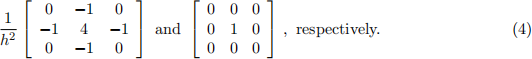
The lexicografic ordering of the grid nodes then leads to the following system of linear equations for the discrete unknowns

for both the interior and the boundary nodes.
Pen and Paper Assignments (50 points)
1. (2 pt) Use Taylor series expansions in the two variables x and y to prove that the local truncation error introduced by the finite difference scheme given by (4) is of second order in the mesh width h (i.e. O(h2)).
2. (3 pt) Assume that N = 3 and therefore h = 1/3. Assume that the boundary conditions are not eliminated from the linear system (5). Assume that the equations corresponding to interior nodes connected to the boundary (i = 2, i = N, j = 2 or j = N) are treated in such a way to keep the matrix Ah symmetric. Give the size of the matrix Ah and the vectors u h and f h . Give all the elements of the matrix Ah and of the vector fh .
3. (5 pt) Derive an expression for the eigenvalues of Ah as a function of h (or equivalently N). It might be advantageous to first compute the eigenvalues of the submatrix of Ah corresponding to the internal nodes.
4. (2 pt) Assume that N = 3 and compute the eigenvalues of Ah numerically. Compare these numerical values with the analytically derived ones in the previous assignment.
5. (6 pt) Show that for all values of h the matrix Ah is an M-matrix. Explain what this means for the convergence of the methods of Jacobi and Gauss-Seidel applied to the system (5).
6. (5 pt) Derive an expression for the eigenvalues of the Jacobi iteration matrix BJAC = Ih − D−1Ah as a function of h (or equivalently N). Here one can exploit the fact that the diagonal of the submatrix of Ah that corresponds to the interior nodes can be written as a constant times the identity matrix of appropriate size. Use these eigenvalues to derive an expression for the asymptotic rate of convergence of the method of Jacobi applied to the system (5) as a function of the mesh width h.
7. (8 pt) Use the red-black ordering of the grid nodes to show that the matrix Ah is consistently ordered. Use the fact that the matrix Ah is consistently ordered to relate the spectral radius of the Gauss-Seidel iteration matrix BGS with that of the Jacobi iteration matrix BJAC. Use this relationship to determine the asymptotic rate of convergence of the Gauss-Seidel method as a function of the mesh width h.
Investigate how the ordering of the grid nodes affects the convergence of the Gauss-Seidel solver. Compare the forward lexicografic, backward lexicografic and red-black ordering of the grid nodes. In a Red-Black ordering all the black nodes are visited only after all the red nodes have been visited. Report your findings.
The convergence of the Gauss-Seidel method can be improved by a convergence acceleration with the help of a coarse grid. In other words: The Gauss-Seidel method will become the smoother in a two-grid algorithm. Verify that the application of the Gauss-Seidel method as a smoother can be written as
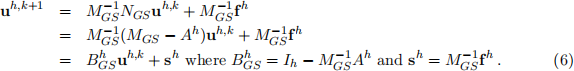
Assume that ν1 and ν2 denote the number of pre and post smoothing steps.
8. (3 pt) Assume that the coarse grid is obtained from the fine grid by standard h → H = 2h coarsening in each coordinate direction as shown in Figure 1. Observe how the boundary is represented on each of the grids. Assume that a vector on the fine grid is restricted to the coarse grid by injection and assume that a vector on the coarse grid is interpolated to the fine grid by bilinear (linear in each coordinate direction) interpolation. Give a stencil representation of the restriction and interpolation operators, I2hh and I2 h h (read symbols from bottom to top), respectively.

Figure 1: Standard coarsening of the fine grid (h) to obtain the coarse grid (2h = H).
9. (4 pt) In a two or three grid method the Gauss-Seidel method assumes the role of the smoother. Investigate how the ordering (lexicografic vs. red-black) affect the smoothing property of the Gauss-Seidel method. Report your findings.
10. (5 pt) Write down a pseudo code for a two-grid V-cycle assuming one pre and one post-smoothing step (i.e., ν1 = 1 and ν2 = 1) and an exact solver on the coarser grid. Use the Gauss-Seidel method as a smoother.
11. (2 pt) Write down the iteration matrix BT GM for the two-grid V-cycle assuming one pre and one post smoothing step on the finest level and a direct solve on the coarsest level.
12. (5 pt) Write down a pseudo code for a three-grid V-cycle and W-cycle assuming again one pre and one post-smoothing step on the finest and intermediate level and a direct solve on the coarsest level.
Implementation Assignments (50 points)
1. (2 pt) Make a plot of the exact solution.
2. (9 pt) Solve the linear system (5) using a direct solver and present in a table ||u h −uex|| (with uex given previously) in the maximum norm (|| · || = maxi | ·i |) for N = 16, 32, 64, 128 and 256. Argue that the computed solution is O(h 2 ) accurate.
Programming assistance:
To detect programming errors it can be useful to plot the difference u h − uex on the mesh employed and to verify whether the error is large on the interior of Ω (possible error in scaling the matrix) or on the boundary Γ (possible error in the treatment of the boundary conditions).
3. (3 pt) Report on how the solution time for the direct solution method used scales with the problem size. Argue to what extent the observed computation times match with the theoretically predicted one.
4. (8 pt) Solve the linear system (5) for N = 16, 32, 64, 128 and 256 using the Gauss-Seidel method as a basic iterative method. Use the forward lexicografic ordering of the grid nodes. Use as initial guess u 0 the constant vector equal to zero. Use as stopping criterion the condition that
∥r k ∥/∥f∥ ≤ T OL = 10−6 . (7)
Make a plot of scaled residuals ∥r k∥/∥f∥ versus k for the various values of N using a logarithmic scale on the y-axis. Report on the number of iterations required to reach convergence as a function of the number N. A measure for the asymptotic speed of convergence is the reduction factor defined as
redk = ||r k ||/||r k−1 || . (8)
Give a table with redk for the last five Gauss-Seidel iterations for the various values of N. Compare this number with the theoretical estimate for the spectral radius of the Gauss-Seidel iteration matrix derived in an earlier assignment.
5. (5 pt) Repeat the previous assignment with the forward lexicografic ordering replaced by the red-black ordering of the grid nodes. Compare the numerical results with the previous assignment. Does this comparison agree with theoretical considerations on the effect of the ordering on the convergence of the solver made earlier? Report your findings.
6. (7 pt) Solve the linear system (5) using the two-grid V-cycle for the various values of N as be-fore. Use the Gauss-Seidel with lexicografic ordering of the grid nodes as a smoother. Use the same starting guess and stopping criterion as before. Present the same convergence statistics (convergence history plot, number of iterations required and asymptotic rate of convergence) as before. Compare these statistics with the ones given in the previous assignments.
7. (5 pt) Repeat the previous assignment with the forward lexicografic ordering replaced by the red-black ordering of the grid nodes. Compare the numerical results with the previous assignment. Does this comparison agree with theoretical considerations on the effect of the ordering on the properties of the Gauss-Seidel used as a smoother? Report your findings.
8. (6 pt) Solve the linear system (5) using the three-grid V-cycle assuming one pre and one post smoothing step for the various values of N as before. Use the Gauss-Seidel method with the lexicografic and red-black ordering as a smoother. Use the same starting guess and stopping criterion as before. Present the same convergence statistics (convergence history plot, number of iterations required and asymptotic rate of convergence) as before. Compare these statistics with the ones given in the previous two assignments.
9. (5 pt) Solve the linear system (5) using the three-grid W-cycle assuming one pre and one post smoothing step for the various values of N as before. Use the same starting guess and stopping criterion as before. Use the Gauss-Seidel method with the lexicografic and red-black ordering as a smoother. Present the same convergence statistics (convergence history plot, number of iterations required and asymptotic rate of convergence) as before. Compare these statistics with the ones given in the previous three assignments.
2024-01-12
Red-Black Two-grid and three-grid iterative method for the discrete Poisson equation