Hello, dear friend, you can consult us at any time if you have any questions, add WeChat: daixieit

MATH3888

Semester 2

Interdisciplinary Project (Streams 1 & 2)

2021

WEEK 8 REPORT GUIDELINES

Submission:

As outlined in the information sheet of this interdisciplinary project course, you will create reports using the (maths) editing software LaTeX:

You are encouraged to use Overleaf to create your LaTeX report which you can access via your browser through your University of Sydney account:

Use the following basic setup for your LaTex file:

Constraints:

The final submitted pdf document shall consist of no more than 4 pages (including figures,....). The ‘fontsize’ is strictly 11 points and the margins of the document are automatically set by the ‘fullpage’ package (as instructed above).

The other package (‘amsmath’) might be needed for the mathematical editing. Add any other packages, if needed.

In addition, you need to submit your Matlab/MatCont source file (*.m, *.mat).

Bifurcation Theory

This week you will check analytic criteria regarding basic bifurcations discussed in previous lectures. Based on that experience you will hopefully appreciate the work MatCont is doing for you.

1. Given the differential equation

(a) Show that (1) undergoes a saddle-node bifurcation, i.e.

i. the ODE (1) possesses an equilibrium state where (i.e. has a zero eigenvalue) and

ii. the map

is regular at .

(Recall: a map is regular at if its linearisation has full rank.)

(b) Based on the regularity of the map in (a)ii, which theorem can you appeal to? Hint: it allows you to conclude explicitly the location of saddle-node points in (µ, x)-space.

(c) Plot a corresponding bifurcation diagram in (µ, x)-space using MatCont. In this problem the curve of equilibria near the saddle-node point can be computed by hand (part (b)): overlay this curve on top of your bifurcation diagram. Hence argue that your numerical work is consistent with your theoretical calculations in (a)–(b).

(d) MatCont also computes a ‘non-degeneracy parameter’ a at the SN point. How does a relate to your calculations? (Hint: look up saddle-node bifurcation on Scholarpedia.)

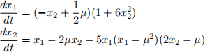
2. Consider the planar system of differential equations dx/dt = f(x, µ), and defined by

(a) Show that (2) undergoes an Andronov-Hopf bifurcation at a bifurcation point , i.e. show that:

i. The eigenvalues of the linearisation at an equilibrium point satisfy and Im (therefore there exists a unique local branch of equilibria parametrised by , with eigenvalues varying smoothly with µ),

ii.

iii.

where denotes the first Lyapunov coefficient.

Note: google the Scholarpedia website on ‘Andronov-Hopf bifurcation’ for how to calculate this coefficient. The planar case is discussed at the very end. Check that your system is in the correct form as stated there. Define the right hand side explicitly that you are using in your calculation.

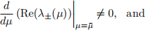
(b) The sign of determines the criticality of the AH-bifurcation. Do you observe a sub- or supercritical AH bifurcation? Hence is the emerging family of limit cycles stable or unstable?

(c) Verify by plotting a corresponding bifurcation diagram in (µ, x1)-space with  using MatCont. Compare your first Lyapunov coefficient computed by hand with the one given numerically by MatCont.