Problem Set 2
Hello, dear friend, you can consult us at any time if you have any questions, add WeChat: daixieit
Problem Set 2 (Due 1pm on December 26, 2023)
Question 1
Consider the following variation of the basic SIR model.
• Ct+1 一 Ct = 一αStCt
• St+1 一 St = αStCt 一 γItSt
• It+1 一 It = γItSt 一 τIt
• Rt+1 一 Rt = τIt
• Ct + St + It + Rt = 1
Set α = 0.02 , γ = 1 , and τ = 0.05 . Assume that C1 = 0.95, S1 = 0.0495, I1 = 0.0005, R1 = 0. Using Matlab, simulate the model from time 1 to time 2,000. Plot the result in a figure with 2-by-2 panels. Ct, St, It, and Rt should be in the top-left, top-right, bottom-left, and bottom- right panels, respectively.
Question 2
Consider the SIRD model considered in the latter part of “Models of Infectious Diseases (II)”.
Find the combination of (i) the state date of the lockdown, (ii) the end date of the lockdown, and (iii) the intensity of the lockdown that maximizes the welfare at time 1, subject to the following restrictions.
. The end date of lockdown is greater than 1 and less than or equal to 200.
. The start date of the lockdown must be less than or equal to the end date of the lockdown.
. α୲ (Intensity of lockdown) takes the same value as long as the lockdown is in place. The set of values that α୲ can take is given by {0, 0.1, 0.2, 0.3, 0.4, 0.5, 0.6, 0.7, 0.8}.
In this exercise, set γ = 0.6, τ = 0.25, κ = 0.02, ϕ = 0.001 . Assume that S1 = 1 一 10-6 , I1 = 10-6 , R1 = 0 , β = 0.99 , and χ = 60,000 . Simulate the model until time 500.
Question 3
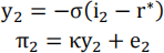
Consider the following log-linearized two-period model with (i) a discounted Euler equation— 0 ≤ α ≤ 1 in front of y2 —, (ii) a forward-looking Phillips curve, (iii) a time-2 cost push shock (e2 ≠ 0) and (iv) no ELB constraint:
At t=1:
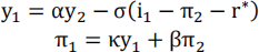
At t=2:
Part A:
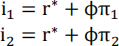
Assume that the policy rate is determined by the Taylor rule:
. Assuming α = 0, solve for (y1, π1, i1, y2, π2, i2) analytically.
Part B:
The government’s per-period utility flow is given by
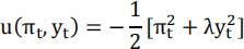
Assume that the government is optimizing under discretion.
. Formulate the optimization problem of the central bank at time 2.
. Formulate the optimization problem of the central bank at time 1.
. Define the Markov-Perfect equilibrium. (You just need to define the equilibrium. You do not need to solve it.)
Part C:
Assume that the government is optimizing under commitment.
. Formulate the optimization problem of the central bank at time 1.
. Define the Ramsey equilibrium. (You just need to define the equilibrium. You do not need to solve it.)
Question 4
Consider the following infinite-horizon loglinearized New Keynesian model with an AR(1) demand shock. Assume that the policy rule is given by an average inflation targeting rule with a 4-quarter window.
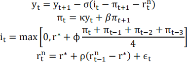
where π0 = π-1 = π-2 = 0. Assume that ϵ < 0 but ϵt = 0 for all time periods after the first period.
Assume the following parameter values: σ = 1, κ = 0.1, β = 1.005/1, r* = 1 - β, ϕ = 5, ρ = 0.7, ϵ1 = 0.015.
Using Dynare, plot the dynamics of y୲ , π୲ , i୲ , and rnt in a figure with 2- by-2 panels.
yt , πt , it , and rnt should be in the top-left, top-right, bottom-left, and bottom-right panels, respectively. In plotting the dynamics, multiply yt by 100 to express it as %., and multiply πt, it, and rt(n) by 400 to express them as annualized %. Adjust fontsize for the figure title, axis labels, and etc. so that it is easy for a reader to understand what the figure shows.
2024-01-11