Hello, dear friend, you can consult us at any time if you have any questions, add WeChat: daixieit

CGP075 Modelling of Chemical Engineering Systems 2023-24

Coursework 2: Simulation and optimisation of water electrolysis for production of “green hydrogen”; individual report and Matlab programs

Summary

For this assignment, you will use Matlab to develop a simulation of the production of hydrogen by electrolysis of water then optimise the operating conditions to achieve maximum efficiency. This case study is based on a published analytical model of water electrolysis for hydrogen production by Xing et al. (2018).1 The work is assessed by report and by the Matlab programs that have been developed.

Objectives

Simulate the efficiency, channel current and furnace potential (an indicator of a temperature constraint being satisfied) and their dependence on temperature, system power and cathode feed ratio.

Investigate and optimise the operating conditions to achieve maximum efficiency.

Explore the performance of the optimisation process and the effect of various optimisation parameters (options) and strategies.

The Model

You will use a slightly simplified version of the model defined for the MPP optimisation in Eq. 37.

System efficiency is defined as

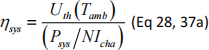
where can be treated as a single variable for this purpose and

.    Calculate the efficiency ηsys and as a function of cathode feed ratio πca

.    Calculate the channel current from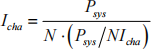

.    Calculate furnace potential Ufur = Uwar + Urea 一 Ucel (Eq 31)

A Matlab function for the calculation of Ucel is provided: “calcCellPotential.m” .

The model can then be investigated at different temperatures and different power levels.

The simplified optimisation can be stated as

subject to constraints

with Ufur,min  = 1.2V and the remaining constraints Eq 37d-f. This optimisation can be studied at different temperatures and power levels. NOTE: your results may not match those in the paper, due   to these simplifications and other approximations e.g. in Ucel . You can adjust Ufur,min  = 1.2V slightly to force the optimisation to proceed successfully if required.

Additional recommendations and hints for the modelling and optimisation

.    Always perform a simulation and explore the system behaviour before attempting to formally optimise the system.

.    Volume fractions of the streams can be taken as mole fractions.

.    When optimising, first perform an unconstrained optimisation, before moving on to include the constraints.

.    You will find it useful to consult Matlab Help files on fmincon, optimoptions, Tolerances and Stopping Criteria, and Tolerance Details amongst others.

.    Use the “interior point” algorithm as recommended in the paper.

.    A stricter compliance with constraints can be achieved by scaling the constraint matrix by multiplying by a large number.

.    You will need to use the functions “assignin” and “evalin” to save and access values    calculated in the model for the constraint function (see example in the crystallisation optimisation programs)

.    Optimisation performance can be affected by e.g. tolerances, the starting point, repeated optimisations (starting from the previous optimised results) etc.

Files Provided

A copy of the paper Xing et al. (2018).

A Matlab function for the calculation of Ucel (“calcCellPotential.m”).

Marking Scheme

This coursework is 50% of the marks for the module.

Report (60% of total for this coursework). The report must be no longer than 6 pages. [Note: valuable information about academic writing can be found in module LUA001 on Learn]

Introduction (5%):

.    the system, its importance, and why modelling and optimisation is relevant.

Simulation (30%)

.     Block diagram of the models (for simulation and optimisation) constructed in Matlab and statement of the functions and settings used.

.     Presentation, analysis and discussion of the results of the model simulating the process.

Optimisation (20%)

.     Mathematical statement of the optimisation, including identification of the objective

function, design variables, constraints (identifying linear and non-linear), and the feasible solution space (lower and upper bounds for the design variables).

.    Analysis of optimisation performance (e.g. convergence) and strategies used to improve it.

.     Presentation, analysis and discussion of the results of the optimisation.

Editorial quality and format (5%)

MATLAB programs (40% of total for this coursework):

Submit your Matlab programs as files. Your code should be well structured, and clearly commented, including reference to Equation numbers or Table numbers in the paper.

Simulation: (25%)

.     implementation of the model as defined in the paper and in this document

.     code for generation of results and their visualisation

Optimisation: (15%)

.     implementation of a formal optimisation using appropriate structures and functions

.    evidence of investigation of optimisation performance improvement strategies and the convergence of the optimisation

.     code for generation and visualisation of optimisation results

Note: all submitted reports will be put through Turnitin (plagiarism detection software). Matlab programs will be checked for evidence of collusion or other forms of academic misconduct.