闪电代写 -代写CS作业_CS代写_Finance代写_Economic代写_Statistics代写_代码代做_IT代写_加急帮助

Hello, dear friend, you can consult us at any time if you have any questions, add WeChat: daixieit

Financial Econometrics, MFE 2023-24

Practical Work 1 (Group Assignment)

Due by 12 noon, 12th January 2024. Upload to SAMS.

IMPORTANT INFORMATION

. This is group work. Groups of three or four are permitted. Groups with less than three or more than four are not permitted.

. All solutions must be submitted by the due date and time: 12 noon, 12th January 2024.

. Do not write the names of members of your group on your submission.

. Candidates should answer all questions.

. Suggested Length: 10 pages.

. Limit: lesser of 15 pages or 3,750 words.

Material on pages 16+ will not be assessed. The limit does not include a cover sheet or academic honesty declaration. All material, including figures, equations, explanatory text, and code, must fit within 15/3,750 words pages.

Assessment

This assignment is assessed in 2 parts:

. 67% - Report: The report should focus on analysis and synthesis and not code or the numerical values of the problems. Tell a convincing story detailing the regularities you have documented in your analysis.

. 33% - Autograder: Two functions must be submitted to compute the required outputs using the inputs. The signature of each function is provided as part of the problem. You must exactly match the function name. Submissions must be in Python and must be in a single Python file (some filename.py) containing all functions. IPython notebooks are not accepted. If using Python, pay close attention to the input and output dimensions. All data inputs will be pandas DataFrames or Series, as indicated in the program description.

Note: Please run your code in the function you submit, to ensure that it does not produce an error. A function that errors when run is given a mark of 0. The autograder uses loose criteria when judging correctness, and so any value within about 1% of the reference will be marked as correct. See the example file solutions-pw1.py for the structure of the file expected by the autograder.

Tips for Autograded Code

. Your submissions MUST be a Python file (.py). IPython notebooks are not accepted, and submit- ting your solution in a notebook will result in a mark of 0.

. Your submission will not have access to any data files. You must not read or write anything from your program.

. Your submission will be run in a random directory. You cannot assume anything about data files existing in any particular location. Your code does not need to access data. All required data is passed through the inputs.

. You can use demo-autograder-pw1.py to check that your solution accepts the required arguments and returns values with the correct type and shape. You should run the program along with your code in an empty directory, which is how the autograder runs it. Code similar to

mkdir empty

cd empty

python demo-autograder-pw1.py

can be used to check that your code will run correctly.

. The autograder submission should not normally have code that you wrote as part of the analysis. It should only contain the required functions, imports, and code necessary to run the functions. An ideal submission would not execute any code when imported, and instead would only contain import statements and functions.

import numpy as np

import pandas as pd

def first_function(a, b):

# Do something

return "something"

def used_by_second_function(x, y):

# Do something

return "something", "else"

def second_function(x, y, z):

w = used_by_second_function(x, y)

return w[0], w[1], z

Problem 1

Data

You will need the following data to complete this assignment:

1. The momentum factor from Ken French’s website (monthly).

2. The 1, 5, and 10-year constant maturity series from FRED.

3. The AAA and BAA (Moody’s) from FRED.

4. The monthly returns on the VWM from Ken French’s site.

5. Monthly data on core CPI from FRED.

6. Monthly data in the unemployment rate from FRED.

7. Monthly data on Industrial Productivity from FRED.

Variable Construction:

1. TERM - The difference between the 10-year and the 1-year

(Y10− Y1).

2. CURVE - The 10-year yield plus the 1-year yield minus 2 times the 5-year yield

Y10− 2Y5 + Y1 = (Y10− Y5) − (Y5− Y1).

3. DEFAULT - The difference between the AAA and the BAA yields

(YAAA− YBAA).

4. INFLATION - The year-over-year difference of log CPI

ln CPIt− ln CPIt−12 .

In-Sample and Out-of-Sample

In-sample exercises should use all available data. Out-of-sample exercises should split the data in half. You will need to construct the common sample of the relevant variables (this may differ between problems 1 and 2). You should construct a single sample where all data is available and only use this common sample.

Analysis

Assess the predictability of the monthly returns of the VWM and the Momentum portfolio, both in-sample and out-of-sample. You should examine the range of available predictors (in the data set constructed).

In particular:

1. Can a predictive model improve the Sharpe ratio in-sample?

2. Is this reproducible out-of-sample?

3. How are in-sample and out-of-sample R2 related?

The “Out-of-sample R2” is defined as

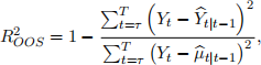
where Yt(~)|t−1 is the model-based forecast of the observation at time t using data up to t−1, and t|t−1 is the sample mean using data up to t−1 (that is, it is the simple mean only forecast). Finally, τ is the starting point of the forecasting exercise. You should consider both univariate regressions using each of the predictors, model-selection-based models (e.g., as selected by the AIC or BIC), and a “kitchen sink” model that uses all predictors. When implementing a model-selection procedure and assessing out-of-sample fit, the selection procedure should be implemented using only the in-sample period.

Note: You may need to time-align observations so that the data for January 2000 is aligned (e.g., the January 2000 unemployment is aligned with the January 2000 return). This is unrealistic since many of these measures are not available in real-time, but it will dramatically simplify the problem.

Notes

The basic regression is

Rt+1 = β0 + β1Xt+ ϵt+1 .

So, the value of R at time t + 1 is determined by the value of X at time t, and the shock ϵ at time t + 1. This is the same whether in-sample or out-of-sample. In-sample means that the same data is used to estimate model parameters as is used to evaluate the model. In this problem, this means th0 1 . Out-of-sample means that estimates of β~0 and β1 use data from 1,...,τ in estimation and then Rτ+1 = β0,τ + β1,τXτ where the notation βj,τ is used to indicate that the estimator is obtained using data until period τ .

Once you have a series of expected returns (either in-sample or out-of-sample), these must be turned into portfolio weights using some function. One example function is

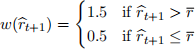
so that when the expected return is above the historical return on would invest 50% more (using leverage) and when it is below one would invest 50% and hold 50% in a risk-free asset. Choosing a weighting function is up to your group. The ultimate quantities to calculate are the portfolio returns

Rp,t+1 = w(R(-)t+1)rt+1+ (1 − w(R(-)t+1))Rf,t+1 .

Importantly, here w(R(-)t+1) is known at time t when using out-of-sample values.

Finally, the portfolio returns can be used to compute the Sharpe ratio in the usual manner. Note that when comparing in-sample and out-of-sample quantities, you should only compare the observations in the common sample (the second half of the sample). It does not make sense to compare a portfolio return or R2 using different time periods.

Problem 2

Data

. Factor returns on the Value and Momentum portfolios from Ken French’s site

. The 6 Portfolios Formed on Size and Momentum

. The 6 Portfolios Formed on Size and Value

. The 17 Industry Portfolios

The Value return is constructed from the 6 Size-Value portfolios as

HML = 1/2(SV + BV) − 1/2(SG + BG)

where S is for small, B is for big, V is for value, and G is for growth. Momentum is similarly defined from the 6 Size-Momentum portfolios as

MOM = 1/2(SH + BH) − 1/2(SL + BL)

where H is high momentum and L is low momentum.

Analysis

1. Critically assess the ability of different model selection procedures to construct accurate out-of- sample tracking portfolios for the Value and Momentum factors using the industry portfolios, as- suming

(a) You train your models using 5-years of data and hold for 5 years;

(b) You train using 10-years of data and then hold for 5 years; and

You should implement these using a 5-year rolling scheme (i.e., estimate using data in 1940-1944, then hold 1945-1949, re-estimate using data in 1945-49, then hold 1950-54, and so on), and only compare samples where all three have predictions available.

2. For each of the two factors considered, examine the ability to track the long-side (the part with positive weights) and the short-side (the part with negative weights) of each factor separately. Comment on the ease or difficulty of replicating the components as opposed to the entire return.

3. Does a combination of your two or three best procedures outperform the components? Note that a combination forecast of n methods is just

where Yi,t+1 is the forecast by method i.

Notes

A tracking regression has the form

where Rp,t is the return on the portfolio being tracked and Ri,t are the returns on assets used to track. There is no constant in this regression.

You can assess the out-of-sample tracking performance by examining the variance of the out-of-sample tracking residuals and comparing these to the out-of-sample variance of the tracked portfolio.

You might want to consider some of GtS and StG (using either p-values or an Information Criterion), Forward Stepwise, Backward Stepwise, or Hybrid Stepwise Procedures, Ridge Regression and LASSO, or Random Forests. It is not expected that you will try them all. A good effort will try a variety of distinct approaches but may have only a few (possibly 1) of each major type.

Code Problems

Out-of-sample R2

Produce a function that will compute the out-of-sample R2 .

r2 = oos_rsquared(y,yhat,mu)

Outputs:

. r2: The out-of-sample R2 (float)

Inputs:

. y: A pandas Series with shape n. The out-of-sample realised value.

. yhat: A pandas Series with shape n. The forecasts of y. The index of yhat will match that of y, so that observation i of yhat will be the forecast of y in position i.

. mu: A float. The in-sample mean of the time-series. Essentially a forecast of y assuming that the correct model has a constant mean.

Out-of-Sample Residual Construction

Compute out-of-sample residuals for values stored in a Series where regressors are a DataFrame and parameters are a Series.

resid = oos_residuals(y, x, beta, first, last)

Outputs:

. resid: A pandas Series with shape n. The value of Y − Xβ for the relevant sample.