MTH6134 Statistical Modelling II Exercises Autumn 2023
Hello, dear friend, you can consult us at any time if you have any questions, add WeChat: daixieit
MTH6134 Statistical Modelling II
Exercises
Autumn 2023
Exercises built upon a list provided by Dr S Coad (formerly of QMUL).
1. Suppose that Yi ∼ Bin(ri , π) for i = 1, 2, . . . , n, all independent, where the ri are known.
1. Write down the likelihood for the data y1, . . . , yn.
2. Find the maximum likelihood estimator ˆπ of π.
3. Prove that ˆπ is an unbiased estimator of π.
2. Suppose you have the following binomial data from a single binomial sample: r = 15, y = 7.
1. Write down the likelihood for the data y.
2. Find the maximum likelihood estimator ˆπ of π.
3. Using R, make a plot of the likelihood function L(π). Examine and describe this function.
4. Consider the following binomial sample: r = 105, y = 49. Repeat the computation of the likelihood L(π), the maximum likelihood estimate ˆπ and the plot of L(π). Compare the results with those of the original data and comment.
3. Consider the following binomial data pairs (r, y): (60, 19),(70, 25),(30, 15),(40, 14),(20, 9).
1. Repeat the computations of steps 1-3 of the previous question (problem 2). In this case, consider and analyze each data pair separately.
2. Analyze the data jointly, using the result of the problem 1.
3. Compare the results of the two analyses. Are the estimates that you obtained related?
4. Suppose that Yi ∼ Poisson(µ) for i = 1, 2, . . . , n, all independent.
1. Write down the likelihood for the data y1, . . . , yn.
2. Find the maximum likelihood estimator ˆµ of µ.
3. Prove that ˆµ is an unbiased estimator of µ.
5. The following count data 5, 1, 3, 5, 5, 4, 3, 2, are assumed to be a series of independent realiza-tions of Poisson(µ).
1. Write down the likelihood for the data y1, . . . , yn.
2. Find the maximum likelihood estimator ˆµ of µ.
3. Plot the likelihood function L(µ) with R. Examine and describe this function.
4. Now suppose that you have a sample of Poisson data with the same sample value ¯y as with the data above, but with n = 16. Redo the plot of L(µ), compare with the first plot and comment.
6. Consider the count data 47, 40, 46, 41, 40. Repeat the computations of items 1-3 of problem 5.
7. Suppose that Yi ∼ N(βxi , σ2 ) for i = 1, 2, . . . , n, all independent, where xi is a known covariate.
1. Write down the likelihood for the data y1, . . . , yn.
2. Find the maximum likelihood estimators βˆ and ˆσ 2 of β and σ 2 .
3. Prove that βˆ is an unbiased estimator of β.
8. In this problem we study properties of the link function g(u) = log(u).
1. Determine the domain and range of g(u).
2. For which type of response is the link g(u) function most suitable?
3. Invert g(u) and compute directly the derivative of the inverse g −1 (u), i.e. du/d g −1 (u).
4. Find out about the inverse function theorem. Use the inverse function theorem to compute the derivative of the inverse g −1 (u).
5. Repeat the steps and computations above for the following link functions:
(a) The identity link g(u) = u.
(b) The inverse quadratic link g(u) = u −2 .
(c) The square root link g(u) = u −1/2 = √ u.
(d) The logit link g(u) = log(u/(1 − u)).
(e) The complementary log-log link g(u) = log(− log(1 − u)).
(f) The Cauchy link g(u) = Φ−1 (u), where Φ(u) = 2/1 + π/1 arctan(u).
(g) (Medium) The Gumbel link g(u) = Φ−1 (u), where Φ(u) = exp(− exp(−u)) is the cumulative Gumbel distribution. Discuss one potential disadvantage of this link.
(h) (Hard) The probit link g(u) = Φ−1 (u), where Φ(u) is the cumulative distribution of the standard normal random variable.
9. Suppose that Yi ∼ N(µ, σ2 ) for i = 1, 2, . . . , n, all independent,
1. Write down the likelihood for the data y1, . . . , yn. Hint: Try to reuse the equations in lecture notes (ditto for the second item).
2. Determine analytically the maximum likelihood estimates.
3. Find the Fisher information matrix.
10. The observations 6.3, 4.2, 6.02, 4.32, 4.04, 3.95 are assumed to be independent realizations of the normal model N(µ, σ2 ).
1. Using R, compute the likelihood estimates with formulæ ˆµ = ¯y and ˆσ 2 = Σni=1(yi −y¯) 2/n.
2. Formulate the estimation of µ, σ like a linear regression in R and compute the estimates ˆµ, ˆσ2 . In other words, use the function lm and process its output.
11. The Federal Trade Commission measured the numbers of milligrammes of tar (x) and carbon monoxide (y) per cigarette for all domestic filtered and mentholated cigarettes of length 100 millimetres. A sample of 12 brands yielded the following data:
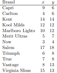
1. Calculate the least squares regression line for these data.
2. Plot the points and the least squares regression line on the same graph.
3. Find an unbiased estimate of σ2.
12. Consider the data on manatees in Practical 1. Use R to answer the questions below.
1. Produce a scatterplot of the data. Does the relationship between y and x seem to be linear?
2. Fit a simple linear regression model to the data. Give the values of βˆ 0 and βˆ 1, and test H0 : β1 = 0.
3. By examining the residual plots, comment on whether there is any reason to doubt the assumptions of the model.
13. Suppose that Yi ∼ N(βxi , σ2 ) for i = 1, 2, . . . , n, all independent, where xi is a known covariate.
1. Find the Fisher information matrix. Hint: Try to reuse the equations in the lecture notes.
2. State the asymptotic distributions of the maximum likelihood estimators βˆ and ˆσ 2 of β and σ 2 .
3. Explain why the distribution of βˆ is exact.
14. Consider the manatees’ data again and a regression model that passes through the origin.
1. Explain in simple terms what does a model going through the origin imply for the mana-tees’ data.
2. Using the data, compute with the help of R an estimate of the matrix V and then give its inverse V −1 which is an estimation of the variance-covariance matrix for the model parameters.
3. Briefly comment upon your results.
15. Consider the model Yi ∼ N(µ, µ2 ) for i = 1, 2, . . . , n, all independent,
1. Write down the likelihood for the data y1, . . . , yn.
2. Determine analytically the maximum likelihood estimate.
3. Find the Fisher information matrix.
16. Suppose that Yi ∼ N(µi , σi 2 ) for i = 1, 2, . . . , n, all independent, where µi = xiβ and the σi are known.
1. Write down the likelihood for the data y1, . . . , yn.
2. Show that βˆ = (X⊤Σ −1X) −1X⊤Σ −1Y is the maximum likelihood estimator of β. Here Σ = diag(σ21, . . . , σ2n).
3. Find the Fisher information matrix.
17. Consider the following data (-1,3.1), (-1,2.1), (0,5.4), (0,4.2), (1,6), (1,6), which is given as pairs (xi , yi). Implement in R the results of the model Yi ∼ N(µi , σ2i) for i = 1, 2, . . . , n, all independent, where µi = β0 + β1xi . The σi are known as σ21 = σ22 = 1, σ23 = σ24 = 2, σ25 = σ26 = 4.
In particular, compute the maximum likelihood estimate βˆ and its asymptotic variance-covariance matrix.
18. Suppose that Yi ∼ Bin(ri , πi) for i = 1, 2, . . . , n, all independent, where the ri are known, πi = β0 + β1xi and xi is a known covariate.
1. Write down the likelihood for the data y1, . . . , yn.
2. Obtain the likelihood equations.
3. Find the Fisher information matrix.
19. Suppose that Yi ∼ Poisson(µi) for i = 1, 2, . . . , n, all independent, where µi = β0 + β1xi and xi is a known covariate.
1. Write down the likelihood for the data y1, . . . , yn.
2. Obtain the likelihood equations.
3. Find the Fisher information matrix.
20. Consider the data on diabetics in Practical 2. Use R to answer the questions below.
1. Produce scatterplots of y against each of the explanatory variables. Does y appear to be linearly related to them?
2. Fit a multiple linear regression model to the full data. Give the values of the estimated regression coefficients and test H0 : β1 = 0.
3. Remove x1 from the model. By examining the residual plots, comment on whether there is any reason to doubt the assumptions of the reduced model.
21. Suppose that Yi ∼ Poisson(µ) for i = 1, 2, . . . , n, all independent, and consider testing H0 : µ = µ0 against H1 : µ ≠ µ0, where µ0 is known.
1. Write down the restricted maximum likelihood estimate ˆµ0 of µ under H0 and the maxi-mum likelihood estimate ˆµ.
2. Obtain the generalised likelihood ratio.
3. Use Wilks’ theorem to find the critical region of a test with approximate significance level α for large n.
22. Consider the data 5, 1, 3, 5, 5, 4, 3, 2 which are assumed to be independent realizations of the Poisson distribution with expectation µ. We want to test H0 : µ = µ0 with µ0 = 3.
1. Obtain the numerical value of the generalised likelihood ratio Λ(y) and discuss about the distribution of this statistic to perform the test H0 : µ = µ0.
2. Use Wilk’s theorem to test H0 : µ = µ0, perform the test and write your conclusions.
3. Using the normal approximation to the data, perform the test H0 : µ = µ0 and compare with the earlier results.
23. Suppose for i = 1, 2, . . . , n, we have independent Yi ∼ Bin(ri , π), where ri is known. Using data y1, . . . , yn, consider testing H0 : p = p0 against H1 : p ≠ p0, where p0 is known.
1. Write down the restricted maximum likelihood estimate ˆp0 of p under H0 and the maxi-mum likelihood estimate ˆp.
2. Obtain the generalised likelihood ratio for this test.
3. Use Wilks’ theorem to find the critical region of a test with approximate significance level α, for large n.
4. The following (25,10), (15,6), (30,10) are data pairs (ri , yi) from acceptance sampling in textile industry. Apply your results to build the generalized likelihood ratio and use Wilks’ theorem with α = 0.05 to test H0 : p = 0.3.
24. Suppose that Y ∼ Bin(r, π), where r is known.
1. Show that this distribution is a member of the exponential family.
2. Explain why the distribution is in canonical form and write down the natural parameter.
3. Use the general results for E{a(Y )} and Var{a(Y )} to verify that E(Y ) = rπ and Var(Y ) = rπ(1 − π).
25. Suppose that Y ∼ N(µ, σ2 ), where σ 2 is known.
1. Show that this distribution is a member of the exponential family.
2. Explain why the distribution is in canonical form and write down the natural parameter.
3. Use the general results for E{a(Y )} and Var{a(Y )} to verify that E(Y ) = µ and Var(Y ) = σ2 .
26. Consider a sequence of independent Bernoulli trials, where each trial has success probability p. The number of failures observed until we obtain r successes is a negative binomial random variable X ∼ NB(r, p) with probability mass function Pr(X = x) = (x+r−1x) p r (1 − p) x .
1. Show that this distribution is a member of the exponential family.
2. Is the distribution in canonical form? Which is the natural parameter?
3. Using exponential family results, show that E(X) = rp/(1 − p).
4. Consider data x1, x2, . . . , xn. Determine the maximum likelihood estimate ˆp. Is this estimator unbiased? Justify your answer.
5. Compute the Fisher information number for estimating p.
27. Consider the random variable Y ∼ Ber(p).
1. Show that this distribution is a member of the exponential family.
2. Determine if the distribution is in canonical form and write down the natural parameter.
3. Use the general results for E{a(Y)} and Var{a(Y)} to determine that E(Y) and Var(Y).
28. Repeat the calculations of Exercise 27 for the following distributions: a) binomial, b) geometric, c) exponential, d) gamma, e) lognormal and f) chi-squared.
29. Consider the mean µ = E(Y ) and variance σ 2 = V (Y ) of the random variable Y ∼ Ber(p). Determine if the variance is a function of the mean and if so, give its explicit formula σ2 = f(µ).
30. Repeat the calculations of Exercise 29 for the following distributions of the exponential family: a) binomial, b) geometric, c) negative binomial, d) Poisson, e) exponential, f) chi-squared, g) gamma and h) lognormal.
31. Suppose that Yi ∼ Bin(ri, πi) for i = 1, 2, . . . , n, all independent, where the ri are known, log{πi/(1 − πi)} = β0 + β1xi and xi is a known covariate.
1. Find the Fisher information matrix.
2. Obtain the asymptotic distributions of the maximum likelihood estimators βˆ0 and βˆ1 of β0 and β1.
3. State the approximate standard errors of βˆ0 and βˆ1.
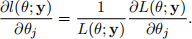
32. Suppose that the continuous random variables Y1, . . . , Yn have distributions depending on the parameters θ1, . . . , θp and that their ranges do not depend on the parameters. Let L(θ; y) and l(θ; y) denote the likelihood and log-likelihood of the parameter vector θ, respectively.
1. Show that
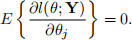
2. Prove that
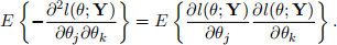
3. By differentiating the identity in part 1 with respect to θk, prove that
2024-01-10