Materials to Teaching Notes of Finance 362
Hello, dear friend, you can consult us at any time if you have any questions, add WeChat: daixieit
Supplementary Materials to Teaching Notes of Finance 362
THE BINOMIAL OPTION PRICING MODEL
Assumptions of the BOPM
The BOPM employs the following assumptions:
1.there are no transaction costs, taxes or margin requirements
2.there are no restrictions on short sales and investors receive the full use of proceeds from short sales
3.securities are infinitely divisible
4.investors can borrow and lend at the riskless interest rate
5.the share price either rises from S to Su or falls from S to Sd over one interval of length Δt (multiplicative binomial process).
6.the riskfree rate, r, is such that 
Pricing one-period European call options on non-dividend shares
Consider a world in which there is a share priced at S on which call options are available. The call option has one period of length A remaining before it expires. Δt expiration date the share will take one of two values, Su (u>1) in the upstate or Sd (d<1) in the downstate.
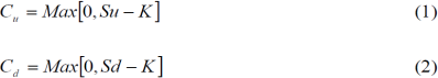
Now consider a call option on the share with an exercise price K and a current price C. On expiration date the call option will be worth its intrinsic value. The intrinsic value of the call will be either Cu in the upstate or Cd in the downstate, where
We now derive a formula for the theoretical price of the option, C, by constructing a riskless portfolio of shares and call options. Note that because the values of a share and a call option on that share move in the same direction we must be long in one and short in the other to create a hedged or riskless investment. Let the riskless portfolio consists of h shares and one written (i.e. short) call option. The current value of this portfolio is defined by:

where S is the current share price and C the current value of the call option.
At expiration the portfolio will be worth either

if the share price rises to Su or

if the share price falls to Sd.
For the portfolio to be riskless the portfolio should have the same end-of-period value regardless of whether the share price rises or falls. That is, Vu = Vd so

Solving equation (6) for h gives

The variable h is referred to as the hedge ratio (or delta). It is measured by the ratio of the high-low spread of the call price to the high-low spread of the share price.
Now the riskless portfolio should earn the riskless rate of return. That is, the end-of-period value of the riskless portfolio should equal its current value compounded for one period at the riskless rate of return. That is,

Note that since the value of the portfolio at expiration is the same whether share prices rise or fall it does not matter whether we use Vu or Vd.
Substituting equation (3) into the LHS of equation (8) and equation (4) into the RHS of equation (8) gives

Rearranging equation (9) gives

Now substituting the formula for the hedge ratio gives
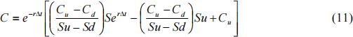
which simplifies to

Equation (12) further simplifies to

where p is defined as
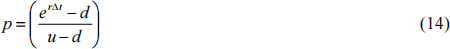
Equation (13) states that the current value of the call option is the present value of the weighted average of the end-of-period payoffs from the option.
Note that the option pricing formulae does not involve the probabilities of the share price moving up or down. For example, we get the same price for the call option when the probability of an uptick is 0.5 as we do when it is 0.9. This seems counterintuitive since we would expect the price of a call option to rise when the probability of an uptick in the share price increases. The reason for this counterintuitive result is that we are not valuing the option in absolute terms but in terms of the price of the underlying share.
The probabilities of future upticks or downticks are already incorporated into the share price. We do not need to take them into account again when valuing the option in terms of the share price.
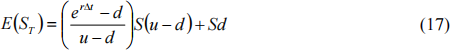
The parameter p is interpreted as the pseudo-probability of an uptick and 1-p as the pseudo-probability of a downtick. Equation (13) can then be interpreted as stating that the current value of a call option is its expected future value discounted at the riskfree rate. The implications of this are as follows. The expected period-end stock price is:

which simplifies to

Substituting equation (14) for p gives
which simplifies to

Equation (18) shows that the share price grows on average at the riskfree rate. Setting the probability of the uptick equal to p is therefore equivalent to assuming that the return on the stock equals the riskfree rate. A world where all investors are risk neutral is referred to as a risk-neutral world. In such a world investors require no compensation for risk and all assets are priced to yield the same riskfree rate of return. This result is an example of the important general principle in option pricing known as risk-neutral valuation.
Option Replication Approach
The call option pricing formulae can be derived by constructing a portfolio of ns shares and B dollars of riskless debt, paying interest r that will replicate the end-of-period payoff of the call option. The initial value of the replicating portfolio is

If S rises to Su, the replicating portfolio must be worth

If S falls to Sd, the replicating portfolio must be worth

Subtracting (3) from (2) gives

which can be rearranged to give

Substituting equation (5) into equation (2)

which simplifies to

Solving equation (7) for B gives
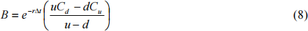
If B is positive the investor is lending at the riskfree rate. If B is negative the investor is borrowing.
Now the expiration date value of the call option is exactly matched by the replicating portfolios value. Therefore, the current value of the call must equal the current value of the replicating portfolio. That is,

Substituting equations (5) and (8) for ns and B in equation (9) yields

which is the same formula derived earlier.
2024-01-04
THE BINOMIAL OPTION PRICING MODEL